Category Archives: Fractals

Image Based Lighting

It can be difficult to achieve realistic lighting by manually placing light sources in a 3D scene. One way to quickly achieve complex and natural lighting is by using real-world light data to lighten the scene.

In order to do that, you need light data from all directions, that is, a full panoramic view. Since you most likely will be looking directly at a light source at some points on your full panorama, you’ll also need to store data that can handle a large dynamic range – 8 bits are not enough.

A common format for these maps is the equirectangular (aka longitude/latitude) format. These are simple 2D bitmaps, typically in 2:1 format, where the x axis covers 360 degrees of azimuthal (longitude) angles, and the y axis covers 180 degrees of elevation (latitude). They are often stored in RGBE (.HDR) files. A good source of free panoramic HDR’s for Image Based Lighting is the sIBL archive.

Backgrounds and reflections

It is very easy to do reflection mapping using equirectangular maps. Simply look up the reflected ray in the equirectangular map. The conversion from 3D direction to map indices is straight-forward:

vec3 equirectangularMap(vec3 dir, sampler2D sampler) {
	// Convert (normalized) dir to spherical coordinates.	
	vec2 longlat = vec2(atan(dir.y,dir.x),acos(dir.z));
	// Normalize, and lookup in equirectangular map.
 	return texture2D(sampler,longlat/vec2(2.0*PI,PI)).xyz;
}

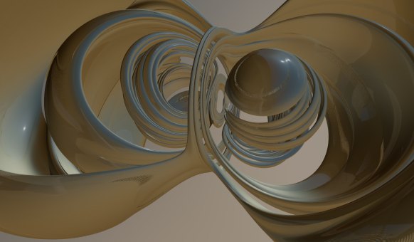
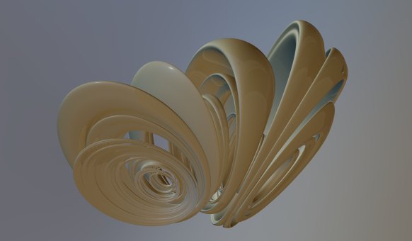
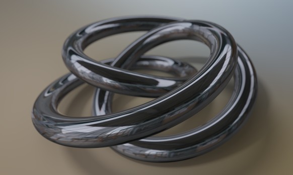
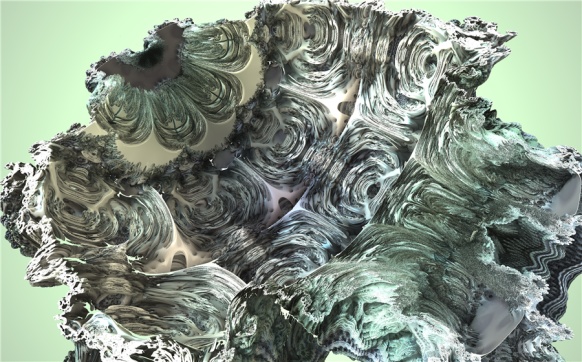
This can also be used to embed the scene in a panoramic view, by looking up the camera ray direction for points that do not hit anything. Here is an example image where reflections and background is sampled from an environment map:

No light model was used in the above image – just pure reflection mapping.

Diffuse light

So what about the diffuse light? Normally, this is modelled by a Lambertian term: the diffuse intensity is proportional to the cosine of the angle between the surface normal and light source direction. In principle, we need to calculate the angle to all points on the hemisphere pointing in the direction of the surface normal, and sum all these contributions. This means, that for each each pixel we raytrace, we need to sample half (one hemisphere) of the pixels in the equirectangular map. Much to slow for even a modern GPU.

But here is the interesting part: the diffuse light contribution is only a function of the surface normal direction. This means we can precalculate the diffuse light in a given normal direction, and store this in a new equirectangular map. Mathematically, this filtering is called a cosine convolution, and some HDR panorama providers are nice enough to provide prefiltered maps for diffuse light (for instance all those in the sIBL archive).

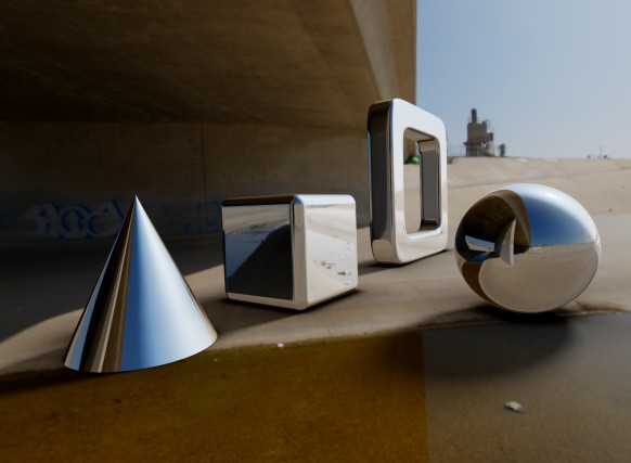
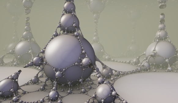
Here is an example of some spheres rendered with specular and diffuse light maps. The materials are faded from pure diffuse (left) to pure specular (right).

As we saw earlier, pure reflection is easy to achieve. But it is also possible to use the Phong reflection model (or other models) with image based lighting. In the Phong model, the specular light intensity depends on the angle between the light source and reflected camera ray. The intensity is proportional to the cosine of this angle raised to a power, which controls the smoothness. Again it is possible to precalculate a convoluted map using the cosine raised to the appropriate power.

Shadows and ground planes

In order to do proper shadows, we would have to check whether the path to every single point on the light map was occluded. Again, this is not feasible. One way to work around this, is to place a single directional light source and then check whether we have a clear to this particular light source. This works nicely, if the light map has a single dominant light source, such as a sun.

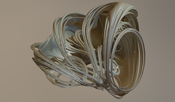
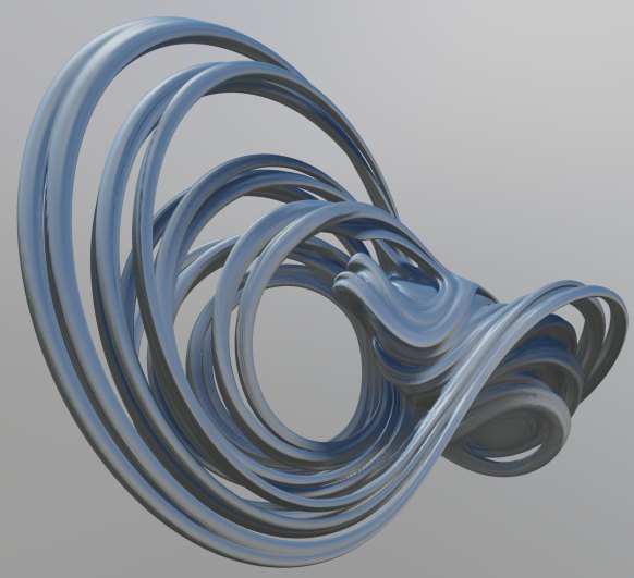
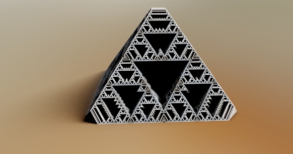
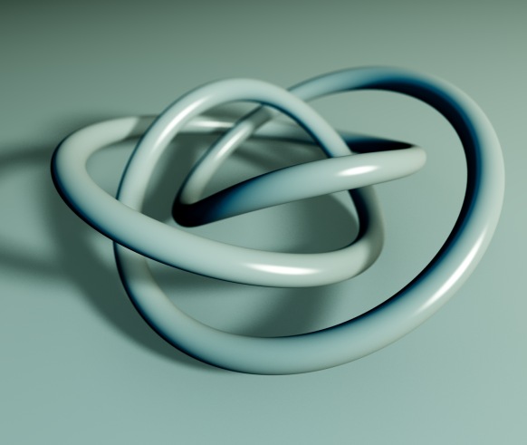
But a problem arise since we do not have any background objects to cast shadows on – the objects in the environment map are placed an infinite distance away, and we don’t know their geometry. Consider this image:

There is no sense of the positioning of the objects in this scene – they seem to float at undefinable locations.

To improve this, we can introduce a ground plane, an invisible object, whose only purpose is to catch shadows.

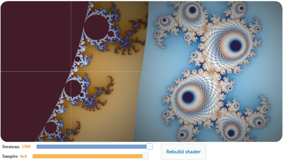
In Fragmentariums IBL-raytracer, you can enable this under the floor tab. It is also possible to turn on some visual debug, to align the floor with the environment map:

Now, once we have set up the ground plane, we can add some ambient occlusion:

… and some shadows:

In order to sample the shadows, we need to sample the area of the light source uniformly. In the case of a sun-like object, this means sampling a hemisphere in a specified direction and for a given latitude span. A formula for this is given in the Global Illumination Compendium (formula 34). To use this, you need to transform the coordinate system to a new one aligned with the light source direction. I do this:

vec3 getSample(vec3 dir, float extent) {
	// Create orthogonal vector (fails for z,y = 0)
	vec3 o1 = normalize(vec3(0., -dir.z, dir.y));
	vec3 o2 = normalize(cross(dir, o1));
	
	// Convert to spherical coords aligned to dir
	vec2 r = getUniformRandomVec2();
	r.x=r.x*2.*PI;
	r.y=1.0-r.y*extent;

	float oneminus = sqrt(1.0-r.y*r.y);
	return cos(r.x)*oneminus*o1+sin(r.x)*oneminus*o2+r.y*dir;
}

Here ‘extent’ is the size of the light source we sample. It is given as ‘1-cos(angle)’, so 0 means a point-like light source (sharp shadows) and 1 means a full hemisphere light source (no shadows).

Notice the construction of the aligned coordinate systems fails if ‘dir’ has zero y and z components – if needed, this should be handled as a special case.

Problems with Simple Image Based Lighting

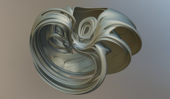
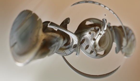
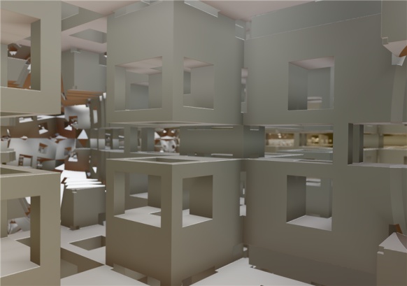
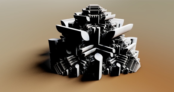
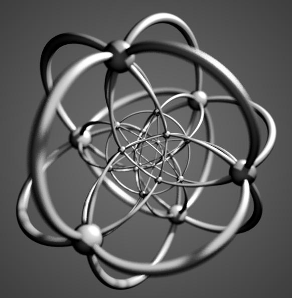
Since no secondary rays are traced for the specular reflections, some geometry ends up with very unrealistic shading:

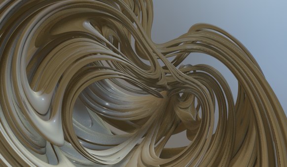
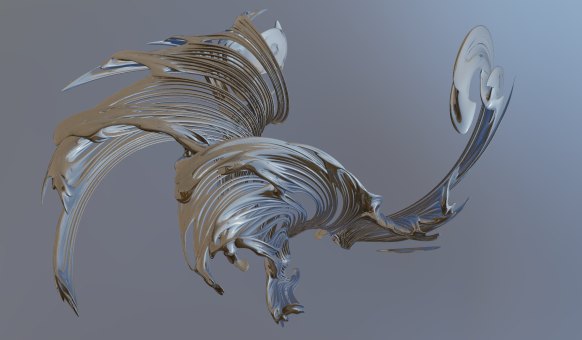
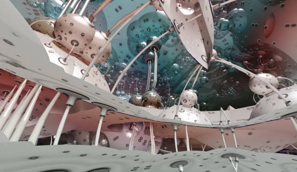
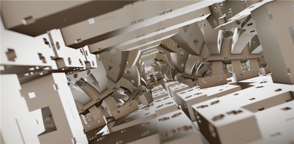
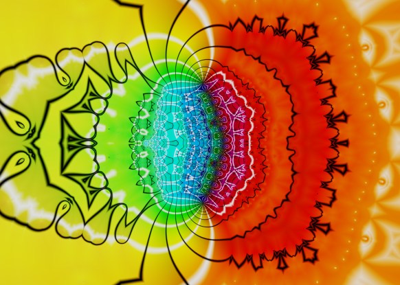
The problems here is that the reflections on the inside on the box sees through the sides. So this simple lighting approach works best for convex objects. Here is another example:

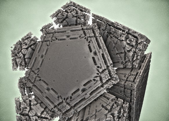
(btw, this is Kali’s dragonKIFS system)

Here again the lighting seems unrealistic – something about the specular light is just wrong.

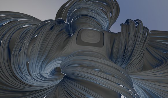
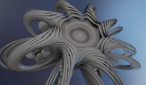
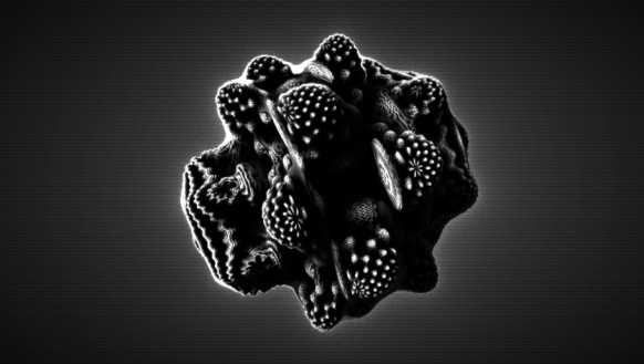
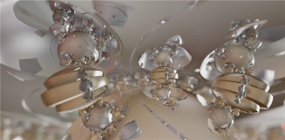
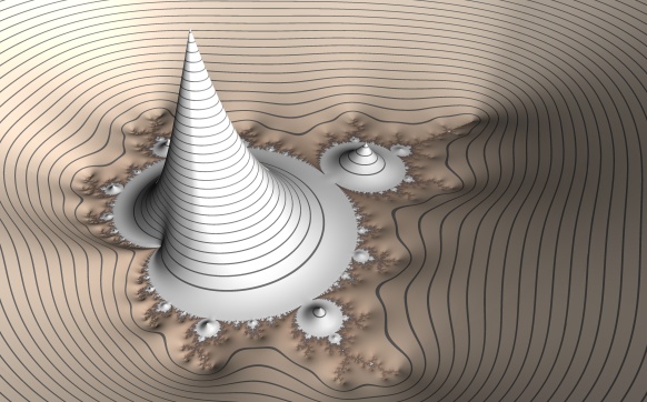
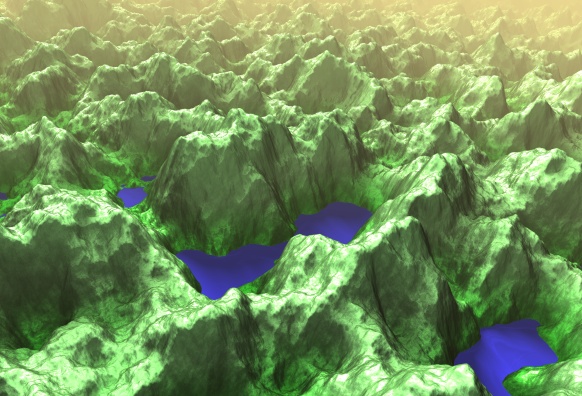
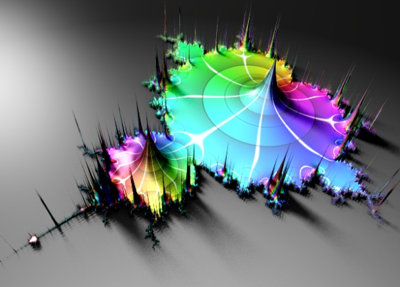
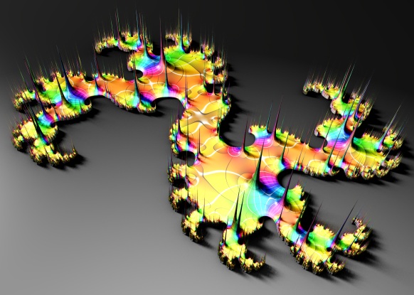
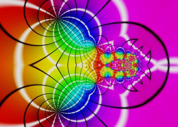
Finally, the combination of the rapidly varying surface normals on a fractal surface and rapidly varying light sources on the environment map introduces new problems. Take a look at this image:

Here there are several small, but strong (HDR) spotlights placed above the Mandelbulb. This image will be very slow to converge and will contain noisy specular highlights: occasionally, one of the subpixel samples will hit a strong light source, which will dominate the sum for the pixel. This will break the sub-pixel anti-aliasing efforts. It is possible to set a maximum (clip) on the specular contributions – or to do HDR tonemapping before averaging – but both solutions goes against the very idea of introducing HDR.

While the specular noise from strong point-like light sources will be difficult to combat, it is easier to do something about the geometry violating reflections.

As of now, I think the best solution is to trace at least secondary rays, and then apply the approximated IBL lighting on the secondary hit points. On problem is that diffuse light does not fall off as quickly as specular light, so you need to sample a lot of points on the hemisphere to get convergence. There are ways around this – for instance, Pixar use bent normals in their Renderman solution, before looking up in the diffuse environment map.

I’ll give a more detailed discussion of the sampling process and the convolution map creation in the next blog post, where I’ll talk about how to speed up diffuse and specular sampling using importance sampling and stratification.

Finally, all the image maps used for lighting on the images accompanying this blog post were from the sIBL archive. And all 3D geometry and composition was of course done in Fragmentarium.

Stereographic Quaternion Julias

Inverse stereographic projections allows you to project a plane onto a sphere. These projections generalize to higher dimensions: for instance, you can inverse project every point in 3D onto the four dimensional 3-sphere. Daniel Piker suggested to use the same transformation to depict the Quaternion Julia systems, instead of using the standard 3D slicing (at least that was what I though – see the update below).

They are still clearly originating from the Quaternions, but the transformation adds a bit of spice. Here are some images:

I’ve previously used stereographic projection to depict Mobius fractals and they were also used to depict the 4D polychora.

For high resolution versions, see my Flickr account.

Update: turns out that what Daniel Piker was suggesting, was to do the stereographic transformation, and then split the 4D coordinates into a starting point and a Julia seed for the ordinary complex (not quaternion) system. I tried this as well, and it creates some very interesting images too:

Rendering 3D fractals without a distance estimator

I have written a lot about distance estimated 3D fractals, and while Distance Estimation is a fast and elegant technique, it is not always possible to derive a distance estimate for a particular system.

So, how do you render a fractal, if the only knowledge you have is whether a given point belongs to the set or not? Or, in other words, how much information can you extract if the only information you have is a black-box function of the form:

bool inside(vec3 point);

I decided to try out some simple brute-force methods to see how they would compare to the DE methods. Contrary to my expectations, it turned out that you can actually get reasonable results without a DE.

First a couple of disclaimers: brute-force methods can not compete with distance estimators in terms of speed. They will typically be a magnitude slower. And if you do have more information available, you should always use it: for instance, even if you can’t find a distance estimator for a given escape time fractal, the escape length contains information that can be used to speed up the rendering or create a surface normal.

The method I used is not novel nor profound: I simply sample random points along the camera ray for each pixel. Whenever a hit is found on the camera ray, the sampling will proceed on only the interval between the camera and the hit point (since we are only interested in finding the closest pixels), e.g. something like this:

for (int i=0; i

(The Near and Far distances are used to restrict the sample space, and speed up rendering)

There are different ways to choose the samples. The simplest is to just sample uniformly (as in the example above), but I found that a stratified approach, where the camera ray segment is divided into equal pieces and a sample is choosen from each part works better. I think the sampling scheme could be improved: in particular once you found a hit, you should probably bias the sampling towards the hit to make convergence faster. Since I use a progressive (double buffered) approach in Fragmentarium, it is also possible to read the pixel depths of adjacent pixels, which probably also could be used.

Now, after sampling the camera rays you end up with a depth map, like this:

(Be sure to render to a texture with 32-bit floats - a 8-bit buffer will cause quantization).

For distance estimated rendering, you can use the gradient of the distance estimator to obtain the surface normal. Unfurtunately this is not an option here. We can, however, calculate a screen space surface normal, based on the depths of adjacent pixels, and transform this normal back into world space:

// Hit position in world space.
vec3 worldPos = Eye + (Near+tex.w*(Far-Near)) * rayDir;

vec3 n = normalize(cross(dFdx(worldPos), dFdy(worldPos)));	

(Update: I found out that GLSL supports finite difference derivatives through the dFdx statement, which made the code above much simpler).

Now we can use a standard lighting scheme, like Phong shading. This really brings a lot of detail to the image:

In order to improve the depth perception, it is possible to apply a screen space ambient occlusion scheme. Recently, there was a very nice tutorial on SSAO on devmaster, but I was to lazy to try it out. Instead I opted for the simplest method I could think of: simply sample some pixels in a neighborhood, and count how many of them that are closer to the camera than the center pixel.

float occ = 0.;
float samples = 0.;
for (float x = -5.; x<=5.; x++) {
  for (float y = -5.; y<=5.; y++) {
    if (x*x+y*y>25.) continue;
    vec3 jitteredPos = pos+vec2(dx*(x+rand(vec2(x,y)+pos)),dy*(y+rand(vec2(x,y)+pos);
    float depth = texture2D(frontbuffer,jitteredPos).w;
    if (depth>=centerDepth) occ+=1.;
    samples++;
  }
}
occ /= samples;

This is how this naive ambient occlusion scheme works:

(Notice that for pixels with no hits, I've choosen to lighten, rather than darken them. This creates an outer glow effect.)

Now combined with the Phong shading we get:

I think it is quite striking how much detail you can infer simply from a depth map! In this case I didn't color the fractal, but nothing prevents you from assigning a calculated color. The depth buffer information only uses the alpha channel.

Here is another example (Aexion's MandelDodecahedron):

While brute-force rendering is much slower than distance estimation, it is possible to render these systems at interactive frame rates in Fragmentarium, especially since responsiveness can be improved by using progressive rendering: do a number of samples, then storing the best found solution (closest pixel) in a depth buffer (I use the alpha channel), render the frame and repeat.

There are a couple of downsides to brute force rendering:

  • It is slower than distance estimation
  • You have to rely on screen space methods for ambient occlusion, surface normals, and depth-of-field
  • Anti-aliasing is more tricky since you cannot accumulate and average. You may render at higher resolution and downsample, or use tiled rendering, but beware that screen space ambient occlusion introduce artifacts which may be visible on tile edges.

On the other hand, there are also advantages:

  • Much simpler to construct
  • Interior renderings are trivial - just reverse the 'inside' function
  • Progressive quality rendering: just keep adding samples, and the image will converge.

To use the Fragmentarium script, just implement an 'inside' function:

#define providesInside
#include "Brute-Raytracer.frag"

bool inside(vec3 pos) {
    // fractal definition here 
}

It is also possible to use the raytracer on existing DE's - here a point is assumed to be inside a fractal if the DE returns a negative number, and outside if the DE returns a positive one.

#include "Brute-Raytracer.frag"

float DE(vec3 pos) {
    // fractal definition here
    // notice, that only the sign of the return value is checked
}

The script can be downloaded as part of Fragmentarium source distribution (it is not yet in the binary distributions). The following files are needed:

Tutorials/3D fractals without a DE.frag
Include/Brute-Raytracer.frag
Include/DepthBufferShader.frag
Include/Brute3D.frag

Fragmentarium Version 0.9.12 (“Prague”) Released

I’ve released a new build of Fragmentarium, version 0.9.12 (“Prague”). It can be downloaded at Github. (Binaries for Windows, source for Windows/Linux/Mac)

The (now standard) caveat apply: Fragmentarium is very much work in progress, and is best suited for people who like to experiment with code.

Version 0.9.12 continues to move Fragmentarium in the direction of progressive HDR rendering. The default raytracers now use accumulated rendering for anti-alias, shadowing, and DOF. To start the progressive rendering, Fragmentarium must be set to ‘Continuous’ mode. It is possible to set a maximum number of rendered frames. All 2D and 3D system now also come with tone mapping, gamma correction, and color control (see the ‘Post’ tab).


IBL Raytracing, using an HDR panorama from Blotchi at HDRLabs.

There is a new raytracer, ‘IBL-raytracer.frag’ which can be used for DE’s instead of the default raytracer. It uses Image Based Lighting from HDR panorama maps. For an example of the new IBL raytracer, see the tutorial: “25 – Image Based Lighting.frag”.

If you need to do stuff like animation, it is still possible to use the old raytracers. They can be included as: “#include “DE-Raytracer-v0.9.1.frag” or “#include “DE-Raytracer-v0.9.10.frag”

Other than that there is now better support for buffer-swap systems (e.g. reaction-diffusion and game-of-life) and better control of texture look-ups.

There are also some interesting new fragments, including the absolutely amazing LivingKIFS.frag script from Kali.

New features

  • Added maximum subframe counter (for progressive rendering).
  • Added support for HDR textures (.hdr RGBE format).
  • Tonemapping, color control, and Gamma correction in buffershader.
  • Added support for widget for changing bound textures.
  • More host defines:
    #define SubframeMax 0
    #define DontClearOnChange   <- when sliders/camera changes, the backbuffer is not cleared.
    #define IterationsBetweenRedraws 20  <- makes it possible to do several steps without updating screen.
    
  • Added texture parameters preprocessor defines:
    #TexParameter texture GL_TEXTURE_MIN_FILTER GL_LINEAR
    #TexParameter texture GL_TEXTURE_MAG_FILTER GL_NEAREST
    #TexParameter texture GL_TEXTURE_WRAP_S GL_CLAMP
    #TexParameter texture GL_TEXTURE_WRAP_T GL_REPEAT
    
  • Change of syntax: when using "#define providesColor", now implement a 'vec3 baseColor(vec3)' function.
  • DE-Raytracer.frag now uses a 'Blinn-Phong with Schickl term and physical normalization'. (Which is something I found in Naty Hoffman's Course Notes).
  • DE-Raytracer.frag and Soft-Raytracer now uses new '3D.frag' base class.
  • Added a texture manager (should reuse and discard textures in memory automatically)
  • Added option to set OpenGL refresh rate in preferences.
  • Progressive2D.frag now supports custom filtering (using '#define providesFiltering')
  • Added support for choosing '#include' through editor context menu.
  • Using arrow keys now work when sliders have focus.
  • Now does a 'reset all' when loading new system (otherwise too confusing).

New fragments

  • Added 'Kali's Creations': KaliBox, LivingKIFS, TreeBroccoli, Xray_KIFS. [Kali]
  • Added Doyle-Spirals.frag [Knighty]
  • Added: Droste.frag (Escher Droste effect)
  • Added: Reaction-Diffusion.frag (Gray-Scott example)
  • Added 'Convolution.frag' example (For precalculating specular and diffuse lighting from HDR panoramas)
  • Added examples of working with double precision floats and emulated double precision floats: "Include/EmulatedDouble.frag", "Theory/Mandelbrot - Emulated Doubles.frag"
  • Added 'IBL-Raytracer.frag' (Image Based Lighting raytracer)
  • Added tutorials: 'progressive2D.frag' and 'pure3D.frag'
  • Added experimental: 'testScene.frag' and 'triplanarTexturing.frag'
  • Added 'Thorn.frag'

Bug fixes

  • Reflection is now working again in 'DE-Raytracer.frag'
  • Fixed filename case sensitivity error when doing reverse lookup of line numbers.

Mac users

Some Mac users has reported problems with the latest versions of Fragmentarium. Again, I don't own a Mac, so I cannot solve these issues without help.

For examples of images generated with the new version, take a look at the Flickr Fragmentarium stream.

Finally, please read the FAQ, before asking questions.

WebGL for Shader Graphics

Web applications are becoming popular, not at least because of Google’s massive effort to push everything through the browser (with Chrome OS being the most extreme example, where everything is running through a browser interface).

Before WebGL, the only way to create efficient graphics was through plug-ins, such as Adobe’s Flash, Microsoft’s Silverlight, Unity, or Google’s O3D and Native Client. But WebGL is a vendor independent technology, directly integrated with the browser’s JavaScript language and DOM model.

Unfortunately, WebGL browser support is limited. WebGL is not available in Internet Explorer on Windows, and is not enabled by default in Safari on Mac OS X. This means that roughly 50% of all internet users won’t have access to WebGL content. WebGL is not supported on iOS devices either (even though it is accessible for iAds, and can be enabled on jail-broken devices).

What is worse, is that Microsoft do not even plan to support WebGL, since they consider it a security threat. Their concerns are reasonable, but their solution is not: it would be much better if they simply showed a dialog box message, warning the user that executing WebGL provides a security risk, and giving a choice to continue or not – the same way they warn about plugins and downloaded executables.

Some very impressive stuff has been done using WebGL, though: for instance ro.me, Path Tracing (Evan Wallace) , Cars (Altered Qualia), Terrain Editor (Rob Chadwick), Traveling Wavefronts (Felix Woitzel), Hartverdrahtet.

Using WebGL for Fractals

There are already some great tools available for experimenting with WebGL: ShaderToy, GLSLSandbox, WebGL Playground. Their main weakness is that it is difficult to store state information (for instance, if you want a movable camera), since this cannot be done in the shader itself, without using weird hacks. So, I decided to start out from scratch to get a feeling for WebGL.

WebGL (specification) is a JavaScript API based on OpenGL ES 2.0, a subset of the desktop OpenGL version designed for embedded devices such as cell phones.

Being a ‘modern’ OpenGL implementation, there is no support for fixed pipeline rendering: there is no matrix stack, no default shaders, no immediate mode rendering (you cannot use glBegin(…) – instead you must use vertex buffers). WebGL also misses some of more advanced features of the desktop OpenGL version, such as 3D textures, multiple render targets, and double precision support. And float texture support is an optional extension.

The first example I made was this Mandelbrot viewer: It demonstrates how to initialise WebGL and compile shaders, render a full-canvas quad, and process keyboard and mouse events and pass them through uniforms to the fragment shader.
Click the image to try out the WebGL demo.

A few programming comments. First JavaScript: I’m not very fond of JavaScript’s type system. The loose typing means that you risk finding bugs later, at run-time, instead of when compiling. It also means that it can be hard to read third-party code (which kind of parameters are you supposed to provide to a function like ‘update(ev, ui)’?). As for numerical types, JavaScript only has the Number type: an IEEE 754 double precision type – no integers!. Some browsers also silently ignore errors during run-time, which makes it even harder to find bugs. On the positive side is the quick iteration time, and the Firebug Firefox plugin, which is an extremely powerful tool for debugging web and JavaScript code.

As for the HTML, I still find it difficult to do table-less layout using floating div’s and css. I’m missing the flexible layout managers that many desktop UI kits provide, which makes it easy to align components and control how they scale when resized (but I may be biased towards desktop UI’s). Also, as HTML was not designed with UI widgets in mind, you have to use a third-party library to display a simple slider: I chose jQuery UI, which was easy to setup and use.

Finally the WebGL: The WebGL GLSL shader code is very similar to the desktop GLSL dialect. The biggest difference is the way loops are handled. Only ‘for’ loops are available, and with a very restricted syntax. It seems the iteration count must be determinable at compilation time (probably because some implementations unroll all loops), which means you no longer can use uniforms to control the loops (you can, however, ‘break’ out of loops dynamically based on run-time variables). This means, that in order to pass the iteration count and number of samples to the Mandelbrot shader, I have to do direct text substitutions in the shader code and recompile.

But my biggest frustation was caused by the ANGLE translation layer. Even for this very simple example, I had several issues with ANGLE – see the notes below.

Feel free to use the example as a starting point for further experiments – it is quite simple to modify the 2D shader code.

Notes about ANGLE

A problem with WebGL is poor graphics driver support for OpenGL. Chrome and Firefox have chosen a very radical approach to solve this: on Windows, they convert all WebGL GLSL shader code into DirectX 9 HLSL code through a converter called ANGLE. Their rationale for doing this, is that OpenGL 2.0 drivers are not available on all computers. However, several shaders won’t run due to the ANGLE translation, and the compilation time can be extremely slow. Wrt drivers, older machines with integrated graphics might be affected, but anything with a less than five year old Nvidia, AMD, or Intel HD graphics card should work with OpenGL 2.0.

In my experiments above, I ran into a bug that in some cases make loops with more than 255 iterations fail (I’ve submitted a bug report).

When debugging ANGLE problems, a good first step is to disable ANGLE and test the shaders. In Chrome, this can be done by starting the executable with the comand line argument –use-gl=desktop. You can check your ANGLE version with the URL chrome://gpu-internals/. In Firefox use the about:config URL, and webgl.force-enabled=true and webgl.prefer-native-gl=true to disable ANGLE.

It is also possible to get the translated HLSL code using the WEBGL_debug_shaders extension. However, this extension is only available for privileged code, which means Chrome must be started with the command line parameter –enable-privileged-webgl-extensions. After that the HLSL source can be obtained by calling:

var hlsl = gl.getExtension("WEBGL_debug_shaders").getTranslatedShaderSource(fragmentShader)

I still haven’t found an workaround for this earlier Mandelbulb experiment (using GLSLSandbox), which fails with another ANGLE bug:
Click the image to try out the WebGL demo (fails on ANGLE systems).

But, I’ll try implementing it from scratch to see if I can find the bug.

Distance Estimated 3D Fractals (Part VIII): Epilogue

This is the last post in my introduction to distance estimated 3D fractals (see Part one for an overview). Originally, I intended this to be much shorter and more focused, but different topics kept sneaking up on me.

This final post discusses hybrid systems, and a few things that didn’t fit naturally in the previous posts. It also contains a small collection of links to relevant resources.

Hybrids

All the fractal systems mentioned in the previous parts apply the same transformation to each point for a number of iterations. But there is nothing that prevents applying different transformations at each iteration step. This has led to a number of hybrid systems, using building blocks from different fractals. They are very popular in Mandelbulb 3D, which comes with a huge library of transformations, which may be stringed together in a vast number of possible combinations.

Spudsville

It is difficult to trace the origin of many of these hybrids, since they are often cloned and modified. One of the more interesting base forms is the Spudsville system by Lenord (see also Hal Tenny’s tutorial on this system).

It is based on the following recipe:

5 x { Mandelbox, i.e. BoxFold, SphereFold, Scaling, Offset }
50 x {BoxFold, Mandelbulb power-2 Squaring }

Pseudo Kleinian

This is another popular base form, based on parameters from Theli-at’s Kleinian Drops. It is based on this formula:

12 x { Scale -1 Mandelbox }
1 x {BoxFold, Mandelbulb power-2 Squaring }
400 x { Scale 2 Mandelbox  }

A version of a similar system is available in Fragmentarium as “Knighty Collection/PseudoKleinian.frag”:

It is also possible to throw some Menger structure into the mix (see “Knighty Collection/PseudoKleinianMenger.frag”):

It is a very diverse system: this is the same formula, that I used as a base form for both Time Pieces:

and Pseudo-Kleinian Blue:

There really is no end to the possibilities. Here is another example:

where an octahedral symmetry transformation has been substituted in a Spudsville-like system:

7 x { Mandelbox, i.e. BoxFold, SphereFold, Scaling, Offset }
7 x { Octahedral, Mandelbulb power-2 Squaring } 

The question is how to construct a suitable distance estimator for these hybrids systems. There is no easy answer to this. Mandelbulb3D and Mandelbulber both use the numerical gradient approximation discussed in part V of this series.

If the system is composed only of conformal transformations, the scalar approach discussed in part VI will be sufficient.

But for general combinations there is no easy way: it is often possible to guess a decent distance estimator, but more often than not, the analytic distance estimator overshoots and needs to be compensated by a fudge factor.

Interior renderings

The Mandelbrot distance estimation formula discussed in part V is only valid for exterior distances. There also exists a formula for the interior distance (for the 2D case), but it is much more complex than the exterior one, since it requires detecting cycles in the orbit.

However, in some cases the exterior distance estimate (or the absolute value of it), also works as an interior estimate (thanks to Visual for pointing this out). Here is an example of the interior of a Mandelbulb:

Geometric Orbit Trapping

Orbit trapping is often used to color fractals. During the orbit calculation the minimum distance to various geometric objects is stored (often the center, a sphere shell, or the x,y, and z-planes).

But it is also possible to use orbit traps to define the geometry of the fractals. Here is a standard Kaleidoscopic IFS like system, defined by DE such as:

float DE(vec3 z)
{
	int n = 0;
	while (n++ < Iterations) {
		// ...do some transformations here
		n++;
	}
	return length(z)*pow(Scale, float(-n));
}

resulting in an image like this:

but by inserting a trap-function and keeping the minimum value, we can create some interesting geometric variations:

float DE(vec3 z)
{
	int n = 0;
	float d= 1000.0;
	while (n++ < Iterations) {
		// ...do some transformations here
		n++;
		d = min(d,  trap(z) * pow(Scale, float(-n)));
	}
	return d;
}

for instance, using a cylinder-function for trap(z) results in an image like this:

Heightmap renderings

It is also possible to use distance estimated methods to draw heightmaps of fractals, e.g.:


Included in Fragmentarium as 'Knighty Collection/MandelbrotHeightField.frag'

Or use heightmaps to visualize the algebraic structure of poles and zeroes in the complex plane:


Included in Fragmentarium as 'Experimental/LiftedDomainColoring3D.frag'

Heightmaps can also be generated from Perlin Noise, to create more realistic terrains:


Included in Fragmentarium as 'Experimental/Terrain.frag'

Knots, Polytopes, and Honeycombs

It is also possible to use distance estimation techniques to depict other mathematical structures than fractals. I've written about them before, but Knighty has explored DE's for knots and polyhedra:

for four-dimensional polychora:

and even for hyperbolic honeycombs:

(There are several examples included with Fragmentarium)

Resources

Software

The easiest way to start exploring 3D fractals is probably by trying Mandelbulb 3D or Mandelbulber. Both are very powerful and feature-rich applications.

Mandelbulb 3D (by Jesse) is probably the most used 3D fractal creation tool (judging by pictures posted at Fractal Forums). It contains many different formulas and fragments, which can be combined as hybrids. It is free, closed-source, CPU-based, and Windows only.

Mandelbulber (by Buddhi) is open source, and available for Windows, Linux, and Mac. CPU-based, but with OpenCL preview!

GPU Based renderers

Fragmentarium is my own playground for working with GPU (GLSL) based pixel graphics. It is meant to create a modular and interactive environment for working with 2D and 3D graphics. All the images in this series of blog post were made with Fragmentarium, and many of the systems are included as examples.

Rrrola's Boxplorer is a fast interactive Mandelbox explorer. It has been extended by Marius Schilder in Boxplorer2 to include spline animations, stereo view, and many examples of fractal systems.

Subblue's Pixel Bender Mandelbulb script was one of the first GPU implementations. He has made many great fractal animations and images, so be sure to visit his web site. He also created the impressive Fractal Lab WebGL site, which made it possible to explore fractals directly in a browser (the site is currently under reconstruction)

Eiffie's Animandel Pro is a tool for creating fractal animations. It features a GLSL editor and even an integrated C-compiler for dynamically compiled CPU code. It is certainly not the easiest way to get started, but as can be seen from Eiffie's videos it is a powerful tool.

Web sites and papers

Fractal Forums is the place, where all the new development and discoveries can be followed. It's a treasure chest filled with information, but it can be difficult to find it in the archives. A good place to start is the original Mandelbox thread and the thread about DE's for the Mandelbox.

Daniel White’s Mandelbulb site is probably the best account of the history of this fractal. Also see Paul Nylander’s Hypercomplex systems.

Tom Lowe's Mandelbox site has a lot of information on the Mandelbox, collected by the person who discovered it himself.

Hypercomplex Iterations: Distance Estimation and Higher Dimensional Fractals (2002). by Dang, Kaufmann, and Sandin is a rare mathematical treatment of higher-dimensional fractals and their distance estimates. It is free (but tough!).

J. C. Hart's original paper Ray tracing deterministic 3-D fractals and his sphere tracing papers are must-reads. He has also written many other great papers.

Pouet.net is a web site for demo scene coders. There is a strong emphasis on heavily optimized and efficient code. Several demos features distance estimation and fractals.

In particular Iñigo Quílez has explored fractals and distance fields in a demo scene context. His Rendering Worlds With Two Triangles is a good introduction to distance field rendering. But be sure to check out Quilez's website - there is an abundance of good stuff, including lots of tutorials.

Spherical Worlds

Recently I saw a description of spherical fractals in a blog post by Samuel Monnier.

These Julia-sets are constructed like ordinary Mandelbrots and Julias: first the argument is squared, but instead of adding a constant afterwards, a Möbius transformation is applied:

\(z = \frac{a z^2 + b}{c z^2 + d}\)

For the right choices of (complex) constants, plane-filling patterns appear.

There is an intimate connection between Möbius transformations and spherical geometry: if the plane is stereographically projected onto a sphere, a Möbius transformations corresponds to rotating and moving the sphere, and then project stereographically back to the plane (this is nicely visualized in this video).


This connection can be visualized graphically: if the plane-filling patterns are stereographically projected onto a sphere, they fit naturally on it. There are no discontinuities or voids, and no singularities near the poles.


Here I’ve used Fragmentarium to create some images of these plane-filling patterns, together with their stereographical projection onto a sphere. It was done by distance estimated ray marching, but in this case we could have used ordinary ray tracing, and calculated the exact intersections.


The Fragmentarium script can be found here.

Lifted Domain Coloring

This year, one of the pictures at the International Science & Engineering Visualization Challenge, caught my interest.

Poelke and Polthier’s Lifted Domain Coloring is a coloring scheme for visualizing properties of complex functions: it maps numbers in the complex plane stereographically to the Riemann sphere, and assigns a hue based on the inclination angle (though I’m not sure that much is gained by the stereographic projection, since the polar representation of the complex numbers seems to provide all the needed information). Saturation and Brightness are controlled by the modulus of the number: when the modulus goes towards infinity, the color turns white, and for numbers close to zero, the color turns black. The exact radial mapping used by the authors is not specified in the paper, but I think my implementation is quite close:

The visualization scheme makes it possible to visually identify different properties, such as zeroes and poles in complex functions.

One of the ways, I think such a visualization may be improved is by using a heightmap:

Here I’ve raised the poles and lowered the zeroes: first, I made the poles and zeroes appear symmetric, by transforming the modulus: r = abs(r + 1/r). Then I applied a sigmoid function to tame the infinities, and finally another sigmoid transformation was applied to change the sign of the zeroes. This technique will only work for somewhat well-behaved functions (meromorph functions – functions with a countable number of zeroes and poles).

Of course, I’ve also tested the Lifted Domain Coloring scheme on fractals.

Here is a Mandelbrot and Julia plot:

Usually Mandelbrot visualizations focus on coloring the outside of the set, but since the exterior of the Mandelbrot set has infinite modulus, only the interior (with its zeroes) are visualized here. The zeroes are visualized as peaks for better graphical clarity.

I also tested the coloring scheme on Samuel Monnier’s Ducks fractal:


Here, the coloring scheme does a decent job for low iteration counts, but for higher iterations the images become messy, so for pure aestethic purposes there are probably better coloring schemes around.

Fragmentarium 0.9 Released

I’ve released a new build of Fragmentarium, version 0.9 (“Sun Ra”).

Download at Github.
(As of now only Windows builds are available)

New features

  • New high resolution output dialog (with auto-naming and auto-backup of scripts and parameters)
  • Locking of parameters (makes rendering considerably faster in some cases by turning uniforms into constants)

Minor improvements

  • Mouse wheel now changes camera position, not FOV
  • Default raytracer improvements:
    • Removed ‘AntiAliasBlur’,’MaxRayStepDiv’, and ‘NormalDetail’ settings
    • Added reflection
    • Shadows (hard, and pseudo-soft shadows)
    • Added dithering (for banding removal) and very simple RNG functionality.
    • Added new ambient occlusion method (similar to Rrola/Subblue – sample along normal for proximity).
  • Added a simpler, but faster version of my raytracer. Just include “Fast-Raytracer.frag” instead of “DE-Raytracer.frag”
  • Added a port of Subblues Fractal Labs (fractal.io) raytracer (GPL). Just include “Subblue-Raytracer.frag” instead of “DE-Raytracer.frag”
  • Added vertical scroll bars to user parameter groups.
  • Added ‘#define providesInit’, ‘#define providesColor’ (to provide custom coloring)
  • Added vec4 GUI slider type
  • Now disables uniforms which are not used in shader.
  • Compiler warnings are now shown in output, also if there is no errors.
  • Bugfix: resize of window now updates aspect ratio.
  • Bugfix: handling of specular exponent = 0
  • BugFix: fixed fps timer for >500ms renders
  • BugFix: Tile Render now works in manual mode.
  • BugFix: Using mouse and key movement at the same time, would result in distance between eye and target getting smaller and smaller.

New fragments

  • A whole collection of new fragments from Knighty!
  • Some of my own new fragments: GraphPlotter, KaliSet, BurningShip, Spudsville, Mandelbrot2D, Terrain.
  • 2DJulia.frag and Complex.frag to make 2D fractals easier.
  • New raytracers: Subblue-Raytracer.frag, Fast-Raytracer.frag
  • QuilezLib with Iñigo Quilez’s collection of sphere tracing primitives
  • Ashima-Noise.frag, a library of Noise functions.

Comments

Some of the new utility libraries make fractals very easy to explore. For instance, 2D escape time fractals are very easy to explore now.

Here is an example:

#include "2DJulia.frag"
#include "Complex.frag"

// 'Ducks' fractal by Samuel Monnier
vec2 formula(vec2 z, vec2 c) {
    return cLog(vec2(z.x,abs(z.y)))+c;
}

which produces this:

Other examples:


Terrain example – example of the new noise library


Mandelbrot heightmap example – based on Knighty’s example

For more example of images generated with the new version, take a look at the Flickr Fragmentarium stream.

Notice for ATI users

Several fragments fail on ATI cards. This seems to be due to faulty GLSL driver optimizations. A workaround is to lock the ‘iterations’ variable (click the padlock next to it). Adding a bailout check inside the main DE loop (e.g. ‘if (length(z)>1000.0) break;’) also seems to do the job.