In some ways path tracing is one of the simplest and most intuitive ways to do ray tracing.
Imagine you want to simulate how the photons from one or more light sources bounce around a scene before reaching a camera. Each time a photon hits a surface, we choose a new randomly reflected direction and continue, adjusting the intensity according to how likely the chosen reflection is. Though this approach works, only a very tiny fraction of paths would terminate at the camera.
So instead, we might start from the camera and trace the ray from here and until we hit a light source. And, if the light source is large and slowly varying (for instance when using Image Based Lighting), this may provide good results.

But if the light source is small, e.g. like the sun, we have the same problem: the chance that we hit a light source using a path of random reflections is very low, and our image will be very noisy and slowly converging. There are ways around this: one way is to trace rays starting from both the camera and the lights, and connect them (bidirectional path tracing), another is to test for possible direct lighting at each surface intersection (this is sometimes called ‘next event estimation’).
Even though the concept of path tracing might be simple, introductions to path tracing often get very mathematical. This blog post is an attempt to introduce path tracing as an operational tool without going through too many formal definitions. The examples are built around Fragmentarium (and thus GLSL) snippets, but the discussion should be quite general.
Let us start by considering how light behaves when hitting a very simple material: a perfect diffuse material.
Diffuse reflections
A Lambertian material is an ideal diffuse material, which has the same radiance when viewed from any angle.

Imagine that a Lambertian surface is hit by a light source. Consider the image above, showing some photons hitting a patch of a surface. By pure geometrical reasoning, we can see that the amount of light that hits this patch of the surface will be proportional to the cosine of the angle between the surface normal and the light ray:
\(
cos(\theta)=\vec{n} \cdot \vec{l}
\)
By definition of a Lambertian material this amount of incoming light will then be reflected with the same probability in all directions.
Now, to find the total light intensity in a given (outgoing) direction, we need to integrate over all possible incoming directions in the hemisphere:
\(
L_{out}(\vec\omega_o) = \int K*L_{in}(\vec\omega_i)cos(\theta)d\vec\omega_i
\)
where K is a constant that determines how much of the incoming light is absorbed in the material, and how much is reflected. Notice, that there must be an upper bound to the value of K – too high a value would mean we emitted more light than we received. This is referred to as the ‘conservation of energy’ constraint, which puts the following bound on K:
\(
\int Kcos(\theta)d\vec\omega_i \leq 1
\)
Since K is a constant, this integral is easy to solve (see e.g. equation 30 here):
\(
K \leq 1/\pi
\)
Instead of using the constant K, when talking about a diffuse materials reflectivity, it is common to use the Albedo, defined as \( Albedo = K\pi \). The Albedo is thus always between 0 and 1 for a physical diffuse materials. Using the Albedo definition, we have:
\(
L_{out}(\vec\omega_o) = \int (Albedo/\pi)*L_{in}(\vec\omega_i)cos(\theta)d\vec\omega_i
\)
The above is the Rendering Equation for a diffuse material. It describes how light scatters at a single point. Our diffuse material is a special case of the more general formula:
\(
L_{out}(\vec\omega_o) = \int BRDF(\vec\omega_i,\vec\omega_o)*L_{in}(\vec\omega_i)cos(\theta)d\vec\omega_i
\)
Where the BRDF (Bidirectional Reflectance Distribution Function) is a function that describes the reflection properties of the given material: i.e. do we have a shiny, metallic surface or a diffuse material.

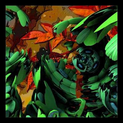
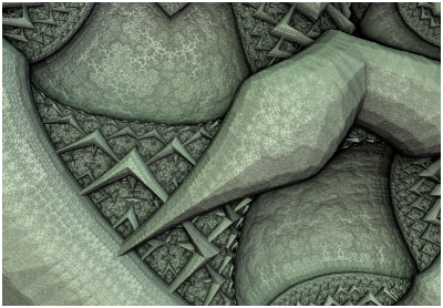
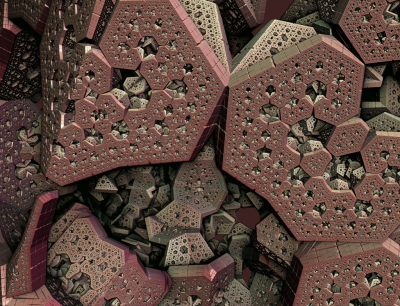
Completely diffuse material (click for large version)
How to solve the rendering equation
An integral is a continuous quantity, which we must turn into something discrete before we can handle it on the computer.
To evaluate the integral, we will use Monte Carlo sampling, which is a very simple: to provide an estimate for an integral, we will take a number of samples and use the average values of these samples multiplied by the integration interval length.
\(
\int_a^b f(x)dx \approx \frac{b-a}{N}\sum _{i=1}^N f(X_i)
\)
If we apply this to our diffuse rendering equation above, we get the following discrete summation:
\begin{align}
L_{out}(\vec\omega_o) &= \int (Albedo/\pi)*L_{in}(\vec\omega_i)cos(\theta)d\vec\omega_i \\
& = \frac{2\pi}{N}\sum_{\vec\omega_i} (\frac{Albedo}{\pi}) L_{in}(\vec\omega_i) (\vec{n} \cdot \vec\omega_i) \\
& = \frac{2 Albedo}{N}\sum_{\vec\omega_i} L_{in}(\vec\omega_i) (\vec{n} \cdot \vec\omega_i)
\end{align}
\)

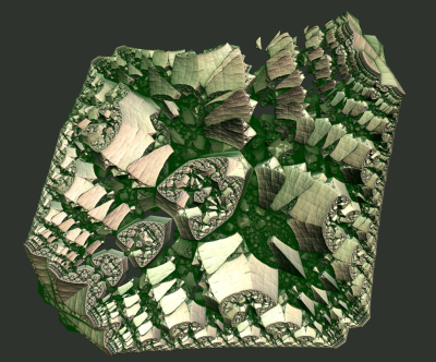
Test render (click for large version)
Building a path tracer (in GLSL)
Now we are able to build a simple path tracer for diffuse materials. All we need to do is to shoot rays starting from the camera, and when a ray hits a surface, we will choose a random direction in the hemisphere defined by the surface normal. We will continue with this until we hit a light source. Each time the ray changes direction, we will modulate the light intensity by the factor found above:
\(
2*Color*Albedo*L_{in}(\vec\omega_i) (\vec{n} \cdot \vec\omega_i)
\)
The idea is to repeat this many times for each pixel, and then average the samples. This is why the sum and the division by N is no longer present in the formula. Also notice, that we have added a (material specific) color. Until now we have assumed that our materials handled all wavelengths the same way, but of course some materials absorb some wavelengths, while reflecting others. We will describe this using a three-component material color, which will modulate the light ray at each surface intersection.
All of this boils down to very few lines of codes:
vec3 color(vec3 from, vec3 dir)
{
  vec3 hit = vec3(0.0);
  vec3 hitNormal = vec3(0.0);

  vec3 luminance = vec3(1.0);
  for (int i=0; i < RayDepth; i++) {
    if (trace(from,dir,hit,hitNormal)) {
       dir = getSample(hitNormal); // new direction (towards light)
       luminance *= getColor()*2.0*Albedo*dot(dir,hitNormal);
       from = hit + hitNormal*minDist*2.0; // new start point
    } else {
       return luminance * getBackground( dir );
    }
  }
  return vec3(0.0); // Ray never reached a light source
}
The getBackground() method simulates the light sources in a given direction (i.e. infinitely far away). As we will see below, this fits nicely together with using Image Based Lighting.
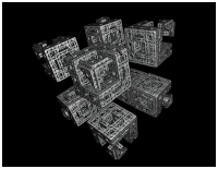
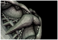
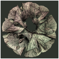
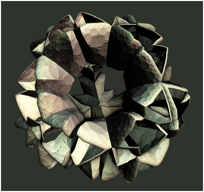
But even when implementing getBackground() as a simple function returning a constant white color, we can get very nice images:

and

The above images were lightened only a constant white dome light, which gives the pure ambient occlusion like renders seen above.
Sampling the hemisphere in GLSL
The code above calls a 'getSample' function to sample the hemisphere.
dir = getSample(hitNormal); // new direction (towards light)
This can be a bit tricky. There is a nice formula for \(cos^n\) sampling of a hemisphere in the GI compendium (equation 36), but you still need to align the hemisphere with the surface normal. And you need to be able to draw uniform random numbers in GLSL, which is not easy.
Below I use the standard approach of putting a seed into a noisy function. The seed should depend on the pixel coordinate and the sample number. Here is some example code:
vec2 seed = viewCoord*(float(subframe)+1.0);

vec2 rand2n() {
    seed+=vec2(-1,1);
	// implementation based on: lumina.sourceforge.net/Tutorials/Noise.html
    return vec2(fract(sin(dot(seed.xy ,vec2(12.9898,78.233))) * 43758.5453),
		fract(cos(dot(seed.xy ,vec2(4.898,7.23))) * 23421.631));
};

vec3 ortho(vec3 v) {
    //  See : http://lolengine.net/blog/2013/09/21/picking-orthogonal-vector-combing-coconuts
    return abs(v.x) > abs(v.z) ? vec3(-v.y, v.x, 0.0)  : vec3(0.0, -v.z, v.y);
}

vec3 getSampleBiased(vec3  dir, float power) {
	dir = normalize(dir);
	vec3 o1 = normalize(ortho(dir));
	vec3 o2 = normalize(cross(dir, o1));
	vec2 r = rand2n();
	r.x=r.x*2.*PI;
	r.y=pow(r.y,1.0/(power+1.0));
	float oneminus = sqrt(1.0-r.y*r.y);
	return cos(r.x)*oneminus*o1+sin(r.x)*oneminus*o2+r.y*dir;
}

vec3 getSample(vec3 dir) {
	return getSampleBiased(dir,0.0); // <- unbiased!
}

vec3 getCosineWeightedSample(vec3 dir) {
	return getSampleBiased(dir,1.0);
}
Importance Sampling
Now there are some tricks to improve the rendering a bit: Looking at the formulas above, it is clear that light sources in the surface normal direction will contribute the most to the final intensity (because of the \( \vec{n} \cdot \vec\omega_i \) term).
This means we might want sample more in the surface normal directions, since these contributions will have a bigger impact on the final average. But wait: we are estimating an integral using Monte Carlo sampling. If we bias the samples towards the higher values, surely our estimate will be too large. It turns out there is a way around that: it is okay to sample using a non-uniform distribution, as long as we divide the sample value by the probability density function (PDF).
Since we know the diffuse term is modulated by the \( \vec{n} \cdot \vec\omega_i = cos(\theta) \), it makes sense to sample from a non-uniform cosine weighted distribution. According to GI compendium (equation 35), this distribution has a PDF of \( cos(\theta) / \pi \), which we must divide by, when using cosine weighted sampling. In comparison, the uniform sampling on the hemisphere we used above, can be thought of either to be multiplied by the integral interval length (\( 2\pi \)), or diving by a constant PDF of \( 1 / 2\pi \).
If we insert this, we end up with a simpler expression for the cosine weighted sampling, since the cosine terms cancel out:
vec3 color(vec3 from, vec3 dir)
{
  vec3 hit = vec3(0.0);
  vec3 hitNormal = vec3(0.0);

  vec3 luminance = vec3(1.0);
  for (int i=0; i < RayDepth; i++) {
    if (trace(from,dir,hit,hitNormal)) {
       dir =getCosineWeightedSample(hitNormal);
       luminance *= getColor()*Albedo;
       from = hit + hitNormal*minDist*2.0; // new start point
    } else {
       return luminance * getBackground( dir );
    }
  }
  return vec3(0.0); // Ray never reached a light source
}
Image Based Lighting
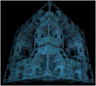
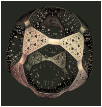
It is now trivial to replace the constant dome light, with Image Based Lighting: just lookup the lighting from a panoramic HDR image in the 'getBackground(dir)' function.
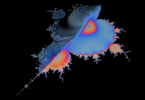
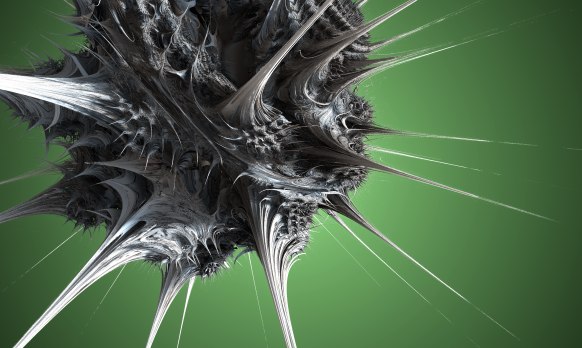
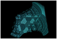
This works nicely, at least if the environment map is not varying too much in light intensity. Here is an example:

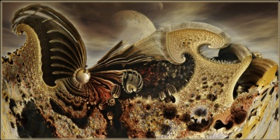
Stereographic 4D Quaternion system (click for large version)
If, however, the environment has small, strong light sources (such as a sun), the path tracing will converge very slowly, since we are not likely to hit these by chance. But for some IBL images this works nicely - I usually use a filtered (blurred) image for lighting, since this will reduce noise a lot (though the result is not physically correct). The sIBL archive has many great free HDR images (the ones named '*_env.hdr' are prefiltered and useful for lighting).
Direct Lighting / Next Event Estimation
But without strong, localized light sources, there will be no cast shadows - only ambient occlusion like contact shadows. So how do we handle strong lights?

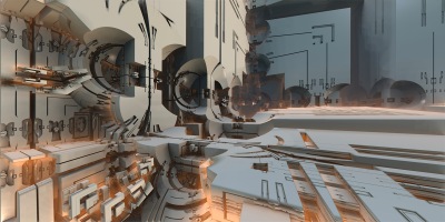
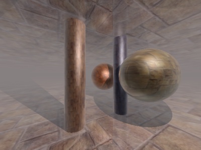
Test scene with IBL lighting
Let us consider the sun for a moment.
The sun has an angular diameter of 32 arc minutes, or roughly 0.5 degrees. How much of the hemisphere is this? The solid angle (which corresponds to the area covered of a unit sphere) is given by:
\(
\Omega = 2\pi (1 - \cos {\theta} )
\)
where \( \theta \) is half the angular diameter. Using this we get that the sun covers roughly \( 6*10^{-5} \) steradians or around 1/100000 of the hemisphere surface. You would actually need around 70000 samples, before there is even a 50% chance of a pixel actually catching some sun light (using \( 1-(1-10^{-5})^{70000} \approx 50\% \)).

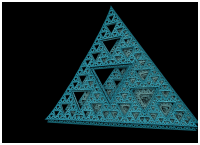
Test scene: naive path tracing of a sun like light source (10000 samples per pixel!)
Obviously, we need to bias the sampling towards the important light sources in the scene - similar to what we did earlier, when we biased the sampling to follow the BRDF distribution.
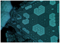
One way to do this, is Direct Lighting or Next Event Estimation sampling. This is a simple extension: instead of tracing the light ray until we hit a light source, we send out a test ray in the direction of the sun light source at each surface intersection.

Test scene with direct lighting (100 samples per pixel)
Here is some example code:
vec3 getConeSample(vec3 dir, float extent) {
        // Formula 34 in GI Compendium
	dir = normalize(dir);
	vec3 o1 = normalize(ortho(dir));
	vec3 o2 = normalize(cross(dir, o1));
	vec2 r =  rand2n();
	r.x=r.x*2.*PI;
	r.y=1.0-r.y*extent;
	float oneminus = sqrt(1.0-r.y*r.y);
	return cos(r.x)*oneminus*o1+sin(r.x)*oneminus*o2+r.y*dir;
}

vec3 color(vec3 from, vec3 dir)
{
  vec3 hit = vec3(0.0);
  vec3 direct = vec3(0.0);
  vec3 hitNormal = vec3(0.0);

  vec3 luminance = vec3(1.0);
  for (int i=0; i < RayDepth; i++) {
    if (trace(from,dir,hit,hitNormal)) {
       dir =getCosineWeightedSample(hitNormal);
       luminance *= getColor()*Albedo;
       from = hit + hitNormal*minDist*2.0; // new start point

       // Direct lighting
       vec3 sunSampleDir = getConeSample(sunDirection,1E-5);
       float sunLight = dot(hitNormal, sunSampleDir);
       if (sunLight>0.0 && !trace(hit + hitNormal*2.0*minDist,sunSampleDir)) {
           direct += luminance*sunLight*1E-5;
       }
    } else {
       return direct + luminance*getBackground( dir );
    }
  }
  return vec3(0.0); // Ray never reached a light source
}
The 1E-5 factor is the hemisphere area covered by the sun. Notice, that you might run into precision errors with the single-precision floats used in GLSL when doing these calculations. For instance, on my graphics card, cos(0.4753 degrees) is exactly equal to 1.0, which means a physically sized sun can easily introduce large numerical errors (remember the sun is roughly 0.5 degrees).
Sky model
To provide somewhat more natural lighting, an easy improvement is to combine the sun light with a blue sky dome.
A slightly more complex model is the Preetham sky model, which is a physically based model, taking different kinds of scattering into account. Based on the code from Simon Wallner I implemented a Preetham model in Fragmentarium.

Here is an animated example, showing how the color of the sun light changes during the day:
Path tracing test from Syntopia (Mikael H. Christensen) on Vimeo.
Fractals
Now finally, we are ready to apply path tracing to fractals. Technically, there is not much new to this - I have previously covered how to do the ray-fractal intersection in this series of blog posts: Distance Estimated 3D fractals.
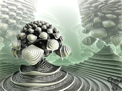
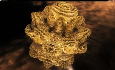
So the big question is whether it makes sense to apply path tracing to fractals, or whether the subtle details of multiple light bounces are lost on the complex fractal surfaces. Here is the Mandelbulb, rendered with the sky model:

Path traced Mandelbulb (click for larger version)
Here path tracing provides a very natural and pleasant lighting, which improves the 3D perceptions.
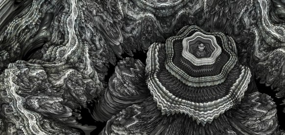
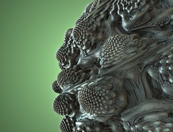
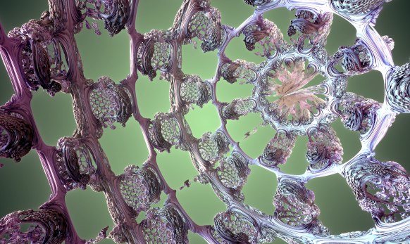
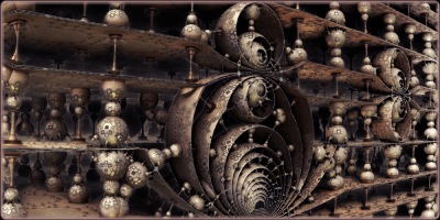
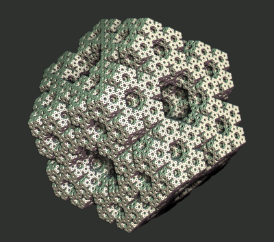
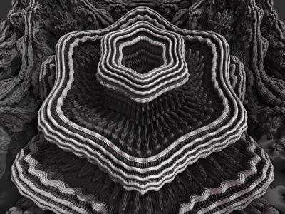
Here are some more comparisons of complex geometry:

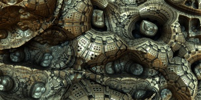
Default ray tracer in Fragmentarium

Path traced in Fragmentarium
And another one:

Default ray tracer in Fragmentarium

Path traced in Fragmentarium
What's the catch?
The main concern with path tracing is of course the rendering speed, which I have not talked much about, mainly because it depends on a lot of factors, making it difficult to give a simple answer.
First of all, the images above are distance estimated fractals, which means they are a lot slower to render than polygons (at least of you have a decent spatial acceleration structure for the polygons, which is surprisingly difficult to implement on a GPU). But let me give some numbers anyway.
In general, the rendering speed will be (roughly) proportional to the number of pixels, the FLOPS of the GPU, and the number of samples per pixel.
On my laptop (a mobile mid-range NVIDIA 850M GPU) the Mandelbulb image above took 5 minutes to render at 2442x1917 resolution (with 100 samples per pixel). The simple test scene above took 30 seconds at the same resolution (with 100 samples per pixel). But remember, that since we can show the render progressively, it is still possible to use this at interactive speeds.
What about the ray lengths (the number of light bounces)?
Here is a comparison as an animated GIF, showing direct light only (the darkest), followed by one internal light bounce, and finally two internal light bounces:

In terms of speed one internal bounce made the render 2.2x slower, while two bounces made it 3.5x slower. It should be noted that the visual effect of adding additional light bounces is normally relatively small - I usually use only a single internal light bounce.
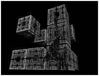
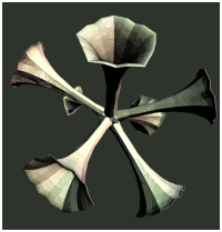
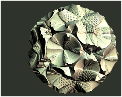
Even though the images above suggests that path tracing is a superior technique, it is also possible to create good looking images in Fragmentarium with the existing ray tracers. For instance, take a look at this image:
(taken from the Knots and Polyhedra series)
It was ray traced using the 'Soft-Raytracer.frag', and I was not able to improve the render using the Path tracer. Having said that, the Soft-Raytracer is also a multi-sample ray tracer which has to use lots of samples to produce the nice noise-free soft shadows.
References
The Fragmentarium path tracers are still Work-In-Progress, but they can be downloaded here:
Sky-Pathtracer.frag (which needs the Preetham model: Sunsky.frag).
and the image based lighting one:
The path tracers can be used by replacing an existing ray tracer '#include' in any Fragmentarium .frag file.
External resources
GI Total Compendium - very valuable collection of all formulas needed for ray tracing.
Vilém Otte's Bachelor Thesis on GPU Path Tracing is a good introduction.
Disney's BRDF explorer - Interactive display of different BRDF models - many examples included. The BRDF definitions are short GLSL snippets making them easy to use in Fragmentarium!
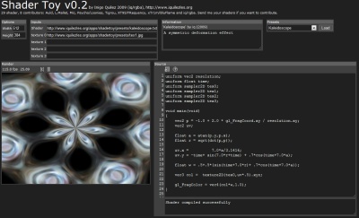
Inigo Quilez's path tracer was the first example I saw of using GPU path tracing of fractals.
Evan Wallace - the first WebGL Path tracer I am aware of.
Brigade is probably the most interesting real time path tracer: Vimeo video and paper.
I would have liked to talk a bit about unbiased and consistent rendering, but I don't understand these issues properly yet. It should be said, however, that since the examples I have given terminate after a fixed number of ray bounces, they will not converge to a true solution of the rendering equation (and, are thus both biased and inconsistent). For consistency, a better termination criterion, such as russian roulette termination, is needed.