Previous posts: part I, part II, part III and part IV.
The last post discussed the distance estimator for the complex 2D Mandelbrot:
(1) \(DE=0.5*ln(r)*r/dr\),
with ‘dr’ being the length of the running (complex) derivative:
(2) \(f’_n(c) = 2f_{n-1}(c)f’_{n-1}(c)+1\)
In John Hart’s paper, he used the exact same form to render a Quaternion system (using four-component Quaternions to keep track of the running derivative). In the paper, Hart never justified why the complex Mandelbrot formula also should be valid for Quaternions. A proof of this was later given by Dang, Kaufmann, and Sandin in the book Hypercomplex Iterations: Distance Estimation and Higher Dimensional Fractals (2002).
I used the same distance estimator formula, when drawing the 3D hypercomplex images in the last post – it seems to be quite generic and applicable to most polynomial escape time fractal. In this post we will take a closer look at how this formula arise.
The Mandelbulb
But first, let us briefly return to the 2D Mandelbrot equation: \(z_{n+1} = z_{n}^2+c\). Now, squaring complex numbers has a simple geometric interpretation: if the complex number is represented in polar coordinates, squaring the number corresponds to squaring the length, and doubling the angle (to the real axis).
This is probably what motivated Daniel Nylander (Twinbee) to investigate what happens when turning to spherical 3D coordinates and squaring the length and doubling the two angles here. This makes it possible to get something like the following object:
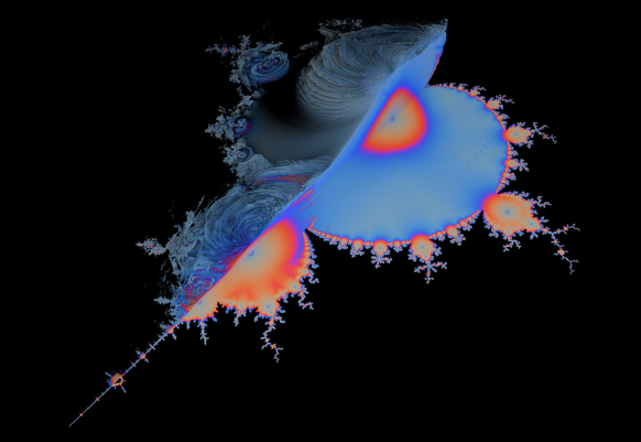
On the image above, I made made some cuts to emphasize the embedded 2D Mandelbrot.
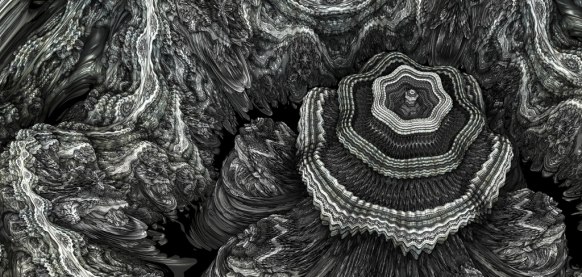
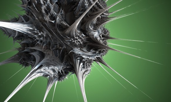
Now, this object is not much more interesting than the triplex and Quaternion Mandelbrot from the last post. But Paul Nylander suggested that the same approach should be used for a power-8 formula instead: \(z_{n+1} = z_{n}^8+c\), something which resulted in what is now known as the Mandelbulb fractal:

The power of eight is somewhat arbitrary here. A power seven or nine object does not look much different, but unexpectedly these higher power objects display a much more interesting structure than their power two counterpart.
Here is some example Mandelbulb code:
float DE(vec3 pos) {
	vec3 z = pos;
	float dr = 1.0;
	float r = 0.0;
	for (int i = 0; i < Iterations ; i++) {
		r = length(z);
		if (r>Bailout) break;

		// convert to polar coordinates
		float theta = acos(z.z/r);
		float phi = atan(z.y,z.x);
		dr =  pow( r, Power-1.0)*Power*dr + 1.0;

		// scale and rotate the point
		float zr = pow( r,Power);
		theta = theta*Power;
		phi = phi*Power;

		// convert back to cartesian coordinates
		z = zr*vec3(sin(theta)*cos(phi), sin(phi)*sin(theta), cos(theta));
		z+=pos;
	}
	return 0.5*log(r)*r/dr;
}
It should be noted, that several versions of the geometric formulas exists. The one above is based on doubling angles for spherical coordinates as they are defined on Wikipedia and is the same version as Quilez has on his site. However, several places this form appears:
float theta = asin( z.z/r );
float phi = atan( z.y,z.x );
...
z = zr*vec3( cos(theta)*cos(phi), cos(theta)*sin(phi), sin(theta) );
which results in a Mandelbulb object where the poles are similar, and where the power-2 version has the nice 2D Mandelbrot look depicted above.
I’ll not say more about the Mandelbulb and its history, because all this is very well documented on Daniel White’s site, but instead continue to discuss various distance estimators for it.
So, how did we arrive at the distance estimator in the code example above?
Following the same approach as for the 4D Quaternion Julia set, we start with our iterative function:
\(f_n(c) = f_{n-1}^8(c) + c, f_0(c) = 0\)
Deriving this function (formally) with respect to c, gives
(3) \(f’_n(c) = 8f_{n-1}^7(c)f’_{n-1}(c)+1\)
where the functions above are ‘triplex’ (3 component) valued. But we haven’t defined how to multiply two spherical triplex numbers. We only know how to square them! And how do we even derive a vector valued function with respect to a vector?
The Jacobian Distance Estimator
Since we have three different function components, which we can derive with three different number components, we end up with nine possible scalar derivatives. These may be arranged in a Jacobian matrix:
\(
J = \begin{bmatrix}
\frac {\partial f_x}{\partial x} & \frac {\partial f_x}{\partial y} & \frac {\partial f_x}{\partial z} \\
\frac {\partial f_y}{\partial x} & \frac {\partial f_y}{\partial y} & \frac {\partial f_y}{\partial z} \\
\frac {\partial f_z}{\partial x} & \frac {\partial f_z}{\partial y} & \frac {\partial f_z}{\partial z}
\end{bmatrix}
\)
The Jacobian behaves like similar to the lower-dimensional derivatives, in the sense that it provides the best linear approximation to F in a neighborhood of p:
(4) \(
F(p+dp) \approx F(p) + J(p)dp
\)
In formula (3) above this means, we have to keep track of a running matrix derivative, and use some kind of norm for this matrix in the final distance estimate (formula 1).
But calculating the Jacobian matrix above analytically is tricky (read the comments below from Knighty and check out his running matrix derivative example in the Quadray thread). Luckily, other solutions exist.
Let us start by considering the complex case once again. Here we also have a two-component function derived by a two-component number. So why isn’t the derivative of a complex number a 2×2 Jacobian matrix?
It turns out that for a complex function to be complex differentiable in every point (holomorphic), it must satisfy the Cauchy Riemann equations. And these equations reduce the four quantities in the 2×2 Jacobian to just two numbers! Notice, that the Cauchy Riemann equations are a consequence of the definition of the complex derivative in a point p: we require that the derivative (the limit of the difference) is the same, no matter from which direction we approach p (see here). Very interestingly, the holomorphic functions are exactly the functions that are conformal (angle preserving) – something which I briefly mentioned (see last part of part III) is considered a key property of fractal transformations.
What if we only considered conformal 3D transformation? This would probably imply that the Jacobian matrix of the transformation would be a scalar times a rotation matrix (see here, but notice they only claim the reverse is true). But since the rotational part of the matrix will not influence the matrix norm, this means we would only need to keep track of the scalar part – a single component running derivative. Now, the Mandelbulb power operation is not a conformal transformation. But even though I cannot explain why, it is still possible to define a scalar derivative.
The Scalar Distance Estimator
It turns out the following running scalar derivative actually works:
(5) \(dr_n = 8|f_{n-1}(c)|^7dr_{n-1}+1\)
where ‘dr’ is a scalar function. I’m not sure who first came up with the idea of using a scalar derivative (but it might be Enforcer, in this thread.) – but it is interesting, that it works so well (it also works in many other cases, including for Quaternion Julia system). Even though I don’t understand why the scalar approach work, there is something comforting about it: remember that the original Mandelbulb was completely defined in terms of the square and addition operators. But in order to use the 3-component running derivative, we need to able to multiply two arbitrary ‘triplex’ numbers! This bothered me, since it is possible to draw the Mandelbulb using e.g. a 3D voxel approach without knowing how to multiply arbitrary numbers, so I believe it should be possible to formulate a DE-approach, that doesn’t use this extra information. And the scalar approach does exactly this.
The escape length gradient approximation
Let us return to formula (1) above:
(1) \(DE=0.5*ln(r)*r/dr\),
The most interesting part is the running derivative ‘dr’. For the fractals encountered so far, we have been able to find analytical running derivatives (both vector and scalar valued), but as we shall see (when we get to the more complex fractals, such as the hybrid systems) it is not always possible to find an analytical formula.
Remember that ‘dr’ is the length of the f'(z) (for complex and Quaternion numbers). In analogy with the complex and quaternion case, the function must be derived with regard to the 3-component number c. Deriving a vector-valued function with regard to a vector quantity suggests the use of a Jacobian matrix. Another approach is to take the gradient of the escape length: \(dr=|\nabla |z_{n}||\) – while it is not clear to me why this is valid, it work in many cases as we will see:
David Makin and Buddhi suggested (in this thread) that instead of trying to calculate a running, analytical derivative, we could use an numerical approximation, and calculate the above mentioned gradient using the finite forwarding method we also used when calculating a surface normal in post II.
The only slightly tricky point is, that the escape length must be evaluated for the same iteration count, otherwise you get artifacts. Here is some example code:
int last = 0;
float escapeLength(in vec3 pos)
{
	vec3 z = pos;
	for( int i=1; i Bailout && last==0) || (i==last))
		{
			last = i;
			return length(z);
		}
	}
	return length(z);
}

float DE(vec3 p) {
	last = 0;
	float r = escapeLength(p);
	if (r*r<Bailout) return 0.0;
	gradient = (vec3(escapeLength(p+xDir*EPS), escapeLength(p+yDir*EPS), escapeLength(p+zDir*EPS))-r)/EPS;
	return 0.5*r*log(r)/length(gradient);
}
Notice the use of the ‘last’ variable to ensure that all escapeLength’s are evaluated at the same iteration count. Also notice that ‘gradient’ is a global varible – this is because we can reuse the normalized gradient as an approximation for our surface normal and save some calculations.
The approach above is used in both Mandelbulber and Mandelbulb 3D for the cases where no analytical solution is known. On Fractal Forums it is usually refered to as the Makin/Buddhi 4-point Delta-DE formula.
The potential gradient approximation
Now we need to step back and take a closer look at the origin of the Mandelbrot distance estimation formula. There is a lot of confusion about this formula, and unfortunately I cannot claim to completely understand all of this myself. But I’m slowly getting to understand bits of it, and want to share what I found out so far:
Let us start by the original Hart paper, which introduced the distance estimation technique for 3D fractals. Hart does not derive the distance estimation formula himself, but notes that:

Now, I haven’t talked about this potential function, G(z), that Hart mentions above, but it is possible to define a potential with the properties that G(Z)=0 inside the Mandelbrot set, and positive outside. This is the first thing that puzzled me: since G(Z) tends toward zero near the border, the “log G(Z)” term, and hence the entire term will become negative! As it turns out, the “log” term in the Hart paper is wrong. (And also notice that his formula (8) is wrong too – he must take the norm of complex function f(z) inside the log function – otherwise the distance will end up being complex too)
In The Science of Fractal Images (which Hart refers to above) the authors arrive at the following formula, which I believe is correct:
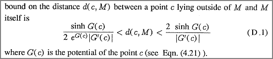
Similar, in Hypercomplex Iterations the authors arrive at the same formula:
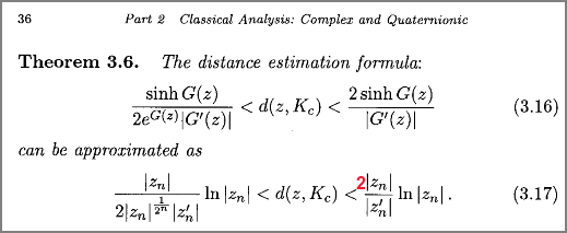
But notice that formula (3.17) is wrong here! I strongly believe it misses a factor two (in their derivation they have \(sinh(z) \approx \frac{z}{2}\) for small z – but this is not correct: \(sinh(z) \approx z\) for small z).
The approximation going from (3.16) to (3.17) is only valid for points close to the boundary (where G(z) approaches zero). This is no big problem, since for points far away we can restrict the maximum DE step, or put the object inside a bounding box, which we intersect before ray marching.
It can be shown that \(|Z_n|^{1/2^n} \to 1\) for \(n \to \infty\). By using this we end up with our well-known formula for the lower bound from above (in a slightly different notation):
(1) \(DE=0.5*ln(r)*r/dr\),
Instead of using the above formula, we can work directly with the potential G(z). For \(n \to \infty\), G(z) may be approximated as \(G(z)=log(|z_n|)/power^n\), where ‘power’ is the polynomial power (8 for Mandelbulb). (This result can be found in e.g. Hypercomplex Iterations p. 37 for quadratic functions)
We will approximate the length of G'(z) as a numerical gradient again. This can be done using the following code:
float potential(in vec3 pos)
{
	vec3 z = pos;
	for(int i=1; i Bailout) return log(length(z))/pow(Power,float(i));
	}
	return 0.0;
}

float DE(vec3 p) {
	float pot = potential(p);
	if (pot==0.0) return 0.0;
	gradient = (vec3(potential(p+xDir*EPS), potential(p+yDir*EPS), potential(p+zDir*EPS))-pot)/EPS;
	return (0.5/exp(pot))*sinh(pot)/length(gradient);
}
Notice, that this time we do not have to evaluate the potential for the same number of iterations. And again we can store the gradient and reuse it as a surface normal (when normalized).
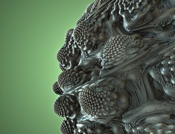
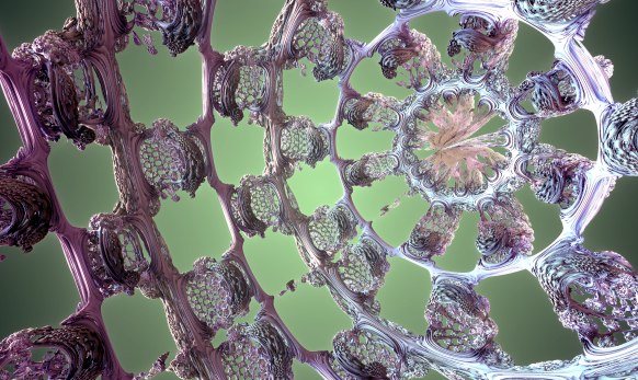
A variant using Subblue’s radiolari tweak
Quilez’ Approximation
I arrived at the formula above after reading Iñigo Quilez’ post about the Mandelbulb. There are many good tips in this post, including a fast trigonometric version, but for me the most interesting part was his DE approach: Quilez used a potential based DE, defined as:
\(DE(z) = \frac{G(z)}{|G'(z)|} \)
This puzzled me, since I couldn’t understand its origin. Quilez offers an explanation in this blog post, where he arrives at the formula by using a linear approximation of G(z) to calculate the distance to its zero-region. I’m not quite sure, why this approximation should be justified, but it seems a bit like an example of Newtons method for root finding. Also, as Quilez himself notes, he is missing a factor 1/2.
But if we start out by formula (3.17) above, and notes that \(sinh(G(z)) \approx G(z)\) for small G(z) (near the fractal boundary) , and that \(|Z_n|^{1/2^n} \to 1\) for \(n \to \infty\) we arrive at:
\(DE(z) = 0.5*\frac{G(z)}{|G'(z)|} \)
(And notice that the same two approximations are used when arriving at our well-known formula (1) at the top of the page).
Quilez’ method can be implemented using the previous code example and replacing the DE return value simply by:
return 0.5*pot/length(gradient);
If you wonder how these different methods compare, here are some informal timings of the various approaches (parameters were adjusted to give roughly identical appearances):
Sinh Potential Gradient (my approach) 1.0x
Potential Gradient (Quilez) 1.1x
Escape Length Gradient (Makin/Buddhi) 1.1x
Analytical 4.1x
The three first methods all use a four-point numerical approximation of the gradient. Since this requires four calls to the iterative function (which is where most of the computational time is spent), they are around four times slower than the analytical solution, that only uses one evaluation.
My approach is slightly slower than the other numerical approaches, but is also less approximated than the others. The numerical approximations do not behave in the same way: the Makin/Buddhi approach seems more sensible to choosing the right EPS size in the numerical approximation of the gradient.
As to which function is best, this requires some more testing on various systems. My guess is, that they will provide somewhat similar results, but this must be investigated further.
The Mandelbulb can also be drawn as a Julia fractal.
Some final notes about Distance Estimators
Mathematical justification: first note, that the formulas above were derived for complex mathematics and quadratic systems (and extended to Quaternions and some higher-dimensional structures in Hypercomplex Iterations). These formulas were never proved for exotic stuff like the Mandelbulb triplex algebra or similar constructs. The derivations above were included to give a hint to the origin and construction of these DE approximations. To truly understand these formula, I think the original papers by Hubbard and Douady, and the works by John Willard Milnor should be consulted – unfortunately I couldn’t find these online. Anyway, I believe a rigorous approach would require the attention of someone with a mathematical background.
Using a lower bound as a distance estimator. The formula (3.17) above defines lower and upper bounds for a given point to the boundary of the Mandelbrot set. Throughout this entire discussion, we have simply used the lower bound as a distance estimate. But a lower bound is not good enough as a distance estimate. This can easily be realized since 0 is always a lower bound of the true distance. In order for our sphere tracing / ray marching approach to work, the lower bound must converge towards to the true distance, as it approaches zero! In our case, we are safe, because we also have an upper bound which is four times the lower bound (in the limit where the exp(G(z)) term disappears). Since the true distance must be between the lower and upper bound, the true distance converges towards the lower bound, as the lower bound get smaller.
DE’s are approximations. All our DE formulas above are only approximations – valid in the limit \(n \to \infty\), and some also only for point close to the fractal boundary. This becomes very apparent when you start rendering these structures – you will often encounter noise and artifacts. Multiplying the DE estimates by a number smaller than 1, may be used to reduce noise (this is the Fudge Factor in Fragmentarium). Another common approach is to oversample – or render images at large sizes and downscale.
Future directions. There is much more to explore and understand about Distance Estimators. For instance, the methods above use four-point numerical gradient estimation, but perhaps the primary camera ray marching could be done using directional derivatives (two point delta estimation), and thus save the four-point sampling for the non-directional stuff (AO, soft shadows, normal estimation). Automatic differentation with dual numbers (as noted in post II) may also be used to avoid the finite difference gradient estimation. It would be nice to have a better understanding of why the scalar gradients work.
The next blog post discusses the Mandelbox fractal.
Another great post and distillation of the various approaches. You’re creating a very useful technical reference here!
I agree with subblue, this is the reference I’ve been looking for since the generalised bulbs first came out 🙂 Thanks again, and I’ll be sure to credit you when I finally get around to implementing it!
Thanks Tom and Thomas!
@Tom: I saw you are updating http://fractal.io/. Really looking forward to see what you will come up with!
All my original formulas (going back to MMFrac in around 2002) used the 2 point directional method (originally based on the difference in smooth iteration values along the rays at step and step+delta) and (even when using the best analytical values rather than just the smooth iteration values) the method suffers from the inherent directionality – if a ray is close to a surface but also parallel to the surface then the DE values are way overestimated because essentially the difference found could be zero. One way to avoid this in 2-point DE is given here:
http://www.fractalforums.com/3d-fractal-generation/true-3d-mandlebrot-type-fractal/msg8604/#msg8604
Hi David, did you also try using the potential G(z)=log(r)/Power^n (the Quilez approach)? It just puzzles me that you cannot use a directional derivative – after all you are only interested in the descent along this path…
Oh, and I just saw at your link that Quilez also tried an Jacobian DE approach. Guess I should be doing some more digging in the Fractal Forums archives 🙂
Awesome articles 🙂
IIRC David Makin and Jos leys had already considered using the jacobian in order to derive an analytical DE. The first analytical DE for the mandelbulb was derived by Jos Leys (using a “vectorial” running derivative see:http://www.fractalforums.com/index.php?topic=742.msg8346#msg8346).
As noted by IQ, the obtained jacobian is a kind of monster. In fact it is possible to split it into a handful of simpler jacobians but this is not the main issue: the analytical jacobian of the mandelbulb suffers from the singularities coming from the transformation to and back from spherical coordinates (the 1/r_xy term). It worsens as iterations number grows. (with one iteration the singularity is along the z axis. with more iterations the z axis singularity is deformed and copied all around. The number of those lines grows exponentially with iteration number).
According to my experiements, using the jacobian (analytically and numerially) to get the gradient of |z_n| using the formula:
grad(z_n) = J(z_n)*z_n/|z_n|
gives hyper noisy renders because of the singularities (BTW the gradient becomes infinite at the singularity lines giving DE=0). I could reduce the noise by using a ridicousely small bailout value (say 1.15 for MB8). A good solution would be to use an hybrid between scalar derivative and Jacobian as You (or subblue?) did with scalar and “vectorial” derivative.
Using the numerical gradient avoids much of the noise but it is still there (the “dendrites”) I guess that the epsilon used in the finite difference formula acts somehow as a smoothing variable. Unfortunately the numerical Jacobian don’t have that feature (or I did it wrong which is highly probable ;))
The scalar and “vectorial” analytic methods don’t have that issue I think just because they neglect the 1/r_xy term.
Concerning “my” method consisting in using the norm of the jacobian, it comes from two observations:
– In the original distance estimation formula approximation (0.5*|z_n|*log(|z_n|)/|z_n’|), z and z’ are complex numbers, which can be represented as matrices (which is also the case of quaternions). It happens that the norm of a complex number coincides with the (euclidean) norm of the matrix representing it.
– In the analytic formula of the gradient: grad(z_n) = J(z_n)*z_n/|z_n|; the gradient is a linear transformation of the unit vector z_n/|z_n|. The definition of the euclidean norm of a matrix M is: max(M.v) where v is a unit vector. Following from that definition : |grad(z_n)| = < |J(z_n)|. That means that if we use the norm of the matrix instead of the norm of the gradient we will get a more conservative DE.
Computing the euclidean matrix norm is quite complicated and ineffective that's why it is better to use other less computationally expensive norms. I've tried successfully "1-norm" and "infinity-norm" with madalabeth, quadray and mandelbox.
In the case of the mandelbox the jacobian and it's norm have (unharmful) discontinuities just like the ones observed when using the gradient. nevertheless the scalar analytical DE gives overall better results for the mandelbox.
Very interesting comment, Knighty! I didn’t know the Jacobian approach was so well studied. It is somewhat unexpected the method is noisy for Mandelbulb – I’d expected it to be the best approximation. Also, the only example I have tried, was your Quadray version, which gave very good results.
Yes, the Jacobian should give the best results. It doesn’t suffer from overstepping around the “flowers” but that come at a price: it is singular when ever z_i comes on the z axis there the norm becomes infinite which imply DE=0. I have no clue on how to “cleanly” remove those singularities. The simplest solution I could imagine is to use the jacobian while z_i is near the fractal’s boundary and the scalar derivatives when it becomes far enought.
For some reason, I was thinking that the formula with sinh() wasn’t usable :/ . Thanks to you, I’ve tried it. It appeared that the 0.5 factor is not necessary. the sinh based formula is closer to the log based one when the 0.5 factor is removed. it seem that the log based formula is the limit case (when G(z)->0) of the lower bound formula but without the 2 in the denominator (or maybe they have defined sinh(x)= exp(x)-exp(-x) instead of sinh(x)= (exp(x)-exp(-x))/2).
Note that IQ’s formula G(z)/|G(z)’| is equivalent to |z_n|*log(|z_n|)/|grad(|z_n|)|. because G(z)=log|z_n|/p^n so grad(G(z))=grad(|z_n|)/p^n/|z_n|. Also, |z_n|^(1/p^n) being equal to exp(G(z)) it tends to 1 when n->infinity but also when distance between z_0 and the fractal tends to 0. When z_0 isn’t “on” the fractal that limit doesn’t hold. For example, the case of the julia with c=0, we have z_n=z_0^(2^n), so |z_n|^(1/2^n)=|z_0|.
Hi, Knighty. If I leave out the”0.5″ term in the DE=0.5/exp(pot))*sinh(pot)/length(gradient), I definitely get overstepping?
I’m not sure which factor 2 you refer to: I think that the lower bounds in formula (3.16) and (3.17) are correct, right? (But with an error of 2 in the upper bound). And in Hypercomplex Iterations, they use ‘sinh(z) -> z/2’ for small z. This would mean they should use sinh(x) = (exp(x)-exp(-x))/4) – I just think it is an error in the book.
I agree that Quilez’s G(z)/|G(z)’| is equivalent to |z_n|*log(|z_n|)/|grad(|z_n|)| (but both are missing a factor 0.5 compared to the lower bound). However, when I try them the Quilez seems to work better: Perhaps taking the numerical gradient of log|z_n| instead of |z_n| improves accuracy? This might matter most on the GPU where we have limited resolution – at least I’ve found the Buddhi/Makin method seems very sensitive to the epsilon step size.
Ooops! You are right. That was a bug in my (evaldraw) script? A classic one: There were two *0.5 and i removed one of them believing there was no *0.5… What a shame! Sorry.
Anyway, I was referring to the lower bound but I was just conjecturing with a false assumption :/
“Hi David, did you also try using the potential G(z)=log(r)/Power^n (the Quilez approach)? It just puzzles me that you cannot use a directional derivative – after all you are only interested in the descent along this path…”
As I said the issue is that using any delta method involving only 2 points will only give you a one-dimensional delta. If you imagine a viewing ray that approaches a section of the fractal that is curving away so as to be parallel to the viewing ray then the delta value will be small resulting in a large DE – at the same location on the ray the 4-point value (or the true analytical value) will still give a “correct” distance *in 3 dimensions*.
The best way to think abut it is to draw a projecting curve in 2D and draw a set of correct DE contour lines around it, these are essentially where the solid boundary will be found using 4-point or analytical DE.
Now imagine a viewing ray heading straight for the point of the projection and imagine using a 2-point delta method to get a DE based on the true DE contours – it will work fine – now try the same thing with a ray approaching at say 90 degrees to the projection point such that it should just strike solid near the end of the projection at the DE threshold for solid – here as the stepping approaches closer the delta value gets too small and produces over-stepping thus when viewed from this angle the end of the projection is missed when it wouldn’t be when using 4-point or analytical.
Even more extreme – imagine a right-angled box section of say a Mandelbox such that a flat side is perpendicular to the viewing plane but immediately behind it or attached to it is a plane parallel to the viewing plane. Rays using the 2 point method traveling close and almost parallel to the “sides” of the box will have very low deltas and thus very high DE’s (because the iteration count/potential etc. essentially are the same at step and step+delta).
Also because of the nature of the 2 point delta method the rendered object will change shape considerably more from one viewpoint to another than will one rendered using a 4-point or analytical method.
Also the method I posted at fractalforums helps to cure various over-stepping issues on Julias even when using 4-point delta or analytical DE.
Love this series of articles and I’m finding them very useful in building my fractal ray marcher. I’ve been playing with the analytic DE method listed in the beginning of the article and I’m having a devil of a time with the surface normals. Previously I’ve been using the SubBlue mandlebulb DE and normal code with great success. When swapping out the DE method I get striping or banding across flat areas of the set that are not present when using the SubBlue DE. The SubBlue normal calculation code is identical to the code presented in a later article in your series. I’ve tweaked just about every parameter I can think of but to no avail. Thank you!
Hi James, have you tried “backstepping” a bit before calculating the normal? It might also be the AO that is causing the banding.
Is there something wrong with this program. I feel like the distance estimator gives total nonsense. Like DE((10000000,10000000,10000000),3) = 1.6038214855339491e-07 ??
def DE(c,q):
z = np.array(c)
dr = 1.0
r = 0.
for i in range(40):
r = np.linalg.norm(z)
dr = (r**(q-1))*q*dr+1
if r>30:
break
p = atan2(z[1],z[0])
t = atan2((z[0]**2 + z[1]**2)**0.5,z[2])
z = (r**q)*np.array([sin(q*t)*cos(q*p),sin(q*t)*sin(q*p),cos(q*t)])
z+=c
return 0.5*log(r)*r/dr