Reaction-diffusion systems model the spatial dynamics of chemicals. An interesting early application was Alan Turing’s theory of Morphogenesis (Turing’s 1951 paper). Here, he suggested, that the pattern formation in animal skin could be explained by a two component reaction-diffusion system.
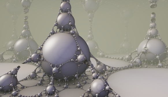
Reaction-diffusion systems are interesting, because they display a wide range of self-organizing patterns, and they have been used by several digital artists, both for 2D pattern generation and 3D structure generation.
The reaction-diffusion model is a great example of how complex large-scale structure may emerge from simple, local rules.
Modelling Reaction-Diffusion on a GPU
As the name suggests, these systems have two driving components: diffusion, which tends to spread out or smoothen concentrations, and reactions, which describe how chemical species may transform into each other.
For each chemical species, it is possible to describe the evolution using a differential equation on the form:
\(\frac {dA}{dt} = K \nabla^2 A + P(A,B)\)
Where A and B are fields describing the concentration of a chemical species at each point in space. The \(K\) coefficient determines how quickly the concentration spreads out, and \(P(A,B)\) is a polynomial in the different species concentrations in the system. There will be a similar equation for the B field.
To model these, we can represent the concentrations on a discrete grid, which fits nicely on a 2D texture on a GPU. The time derivative can solved in discrete time steps using forward Euler integration (or something more powerful). On a GPU, we need two buffers to do this: we render the next time step into the front buffer using values from the back buffer, and then swap the buffers.
Buffer swapping is a standard technique, and in Fragmentarium the only thing you need to do, is to declare a ‘uniform sampler2D backbuffer;’ and Fragmentarium will take care of creation and swapping of buffers. We also use the Fragmentarium host define ‘#buffer RGBA32F’ to ask for four-component 32-bit float buffers, instead of the normal 8-bit integer buffers.
The Laplacian may be calculated using a finite differencing scheme, for instance using a five-point stencil:
vec3 P = vec3(pixelSize, 0.0);

// Five point stencil Laplacian
vec4  laplacian5() {
	return
	+  texture2D( backbuffer, position - P.zy)
	+  texture2D( backbuffer, position - P.xz)
	-  4.0 * texture2D( backbuffer,  position )
	+ texture2D( backbuffer,  position + P.xz )
	+ texture2D( backbuffer,  position +  P.zy );
}
(see the Fragmentarium source for a nine-point stencil).
A simple two-component Gray-Scott system may then be modelled simply as:
// time step for Gray-Scott system:
vec4 v = texture2D(backbuffer, position);
vec2 lv = laplacian5().xy; // laplacian
float xyy = v.x*v.y*v.y;   // utility term
vec2 dV = vec2( Diffusion.x * lv.x - xyy + f*(1.-v.x), Diffusion.y * lv.y + xyy - (f+k)*v.y);
v.xy += timeStep*dV;
(Robert Munafo has a great page with more information on Gray-Scott systems).
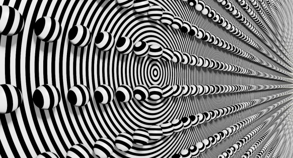
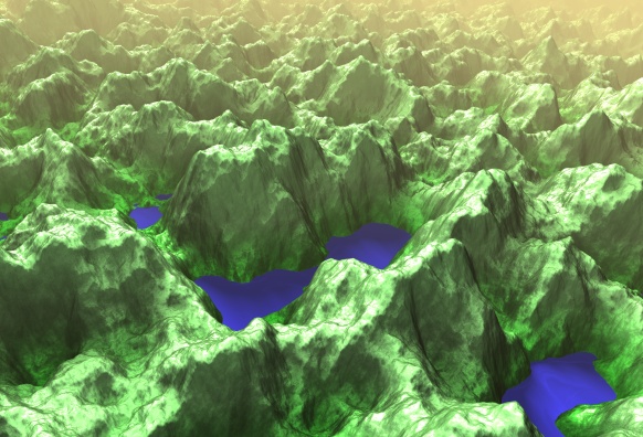
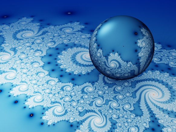
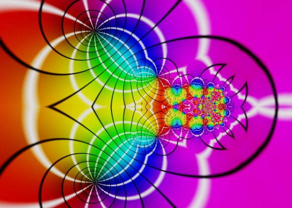
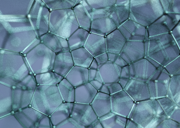
Here is an example of a typical system created using the above system, though many other patterns are possible:

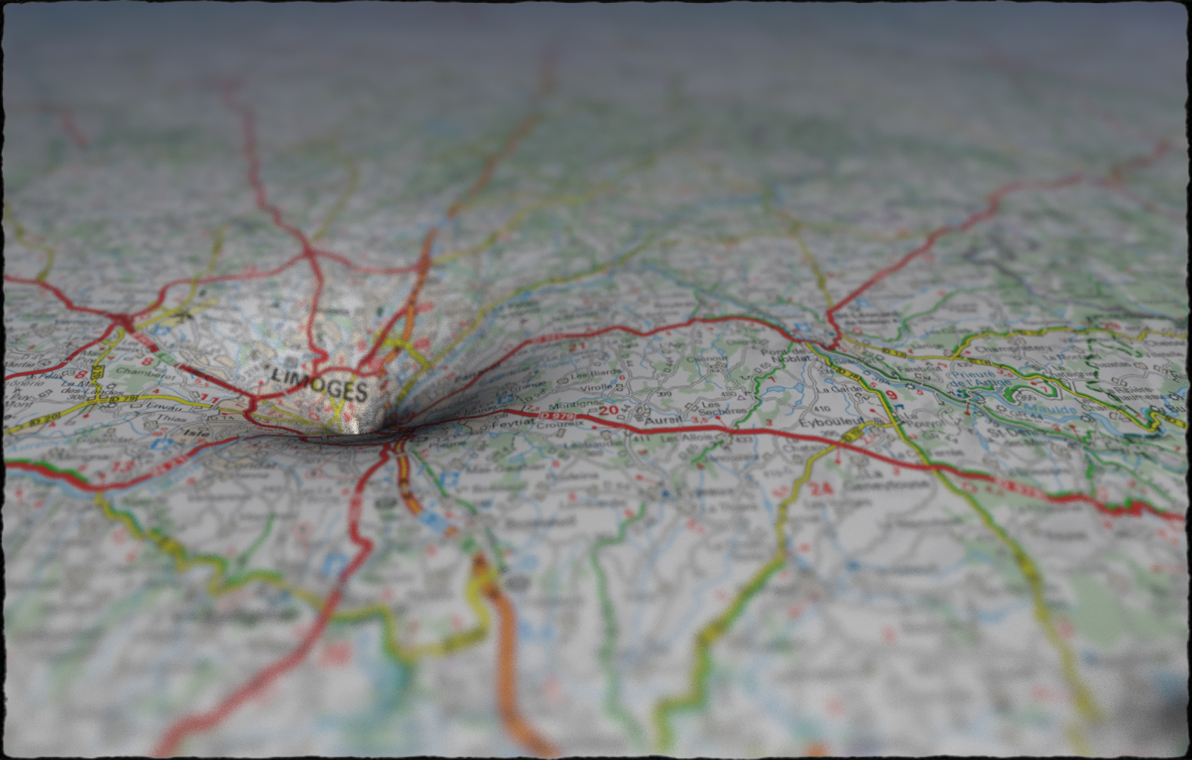
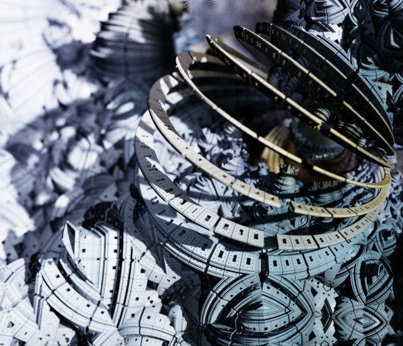
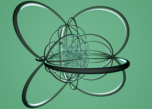
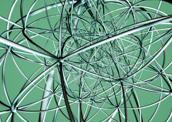
It is also possible to enforce some structure by changing the concentrations in certain regions:

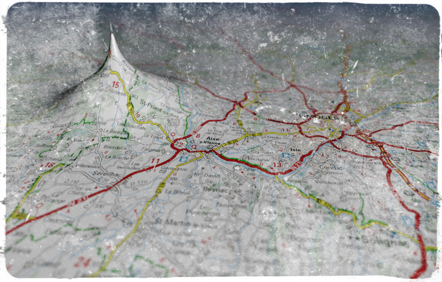
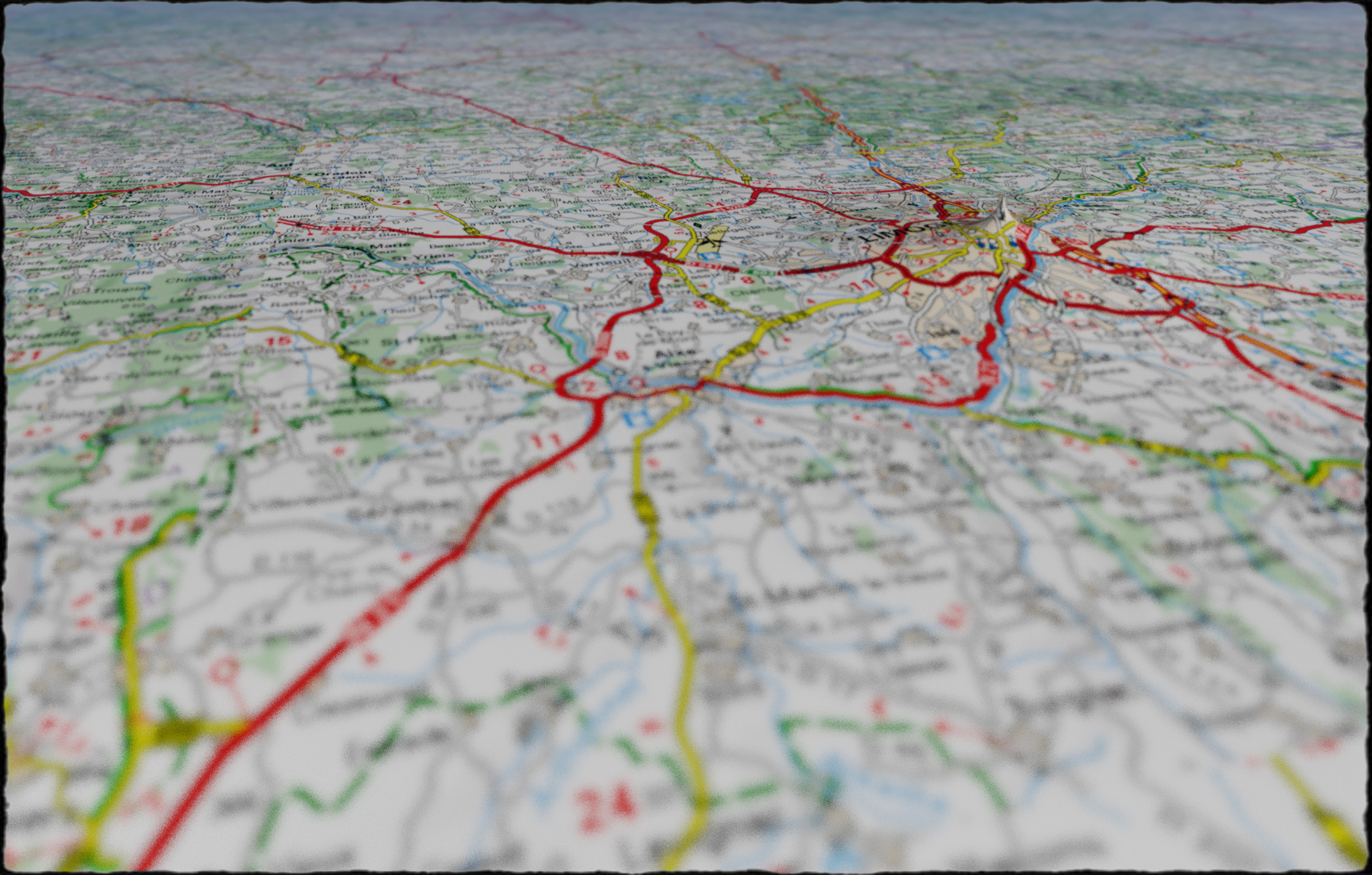
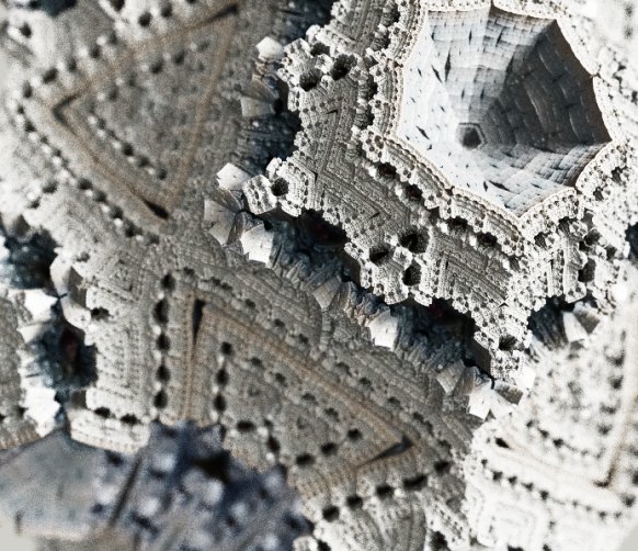
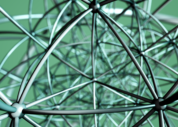
You can even use a picture to modify the concentrations:

A template implementation can be found as part of the Fragmentarium source at GitHub: Reaction-Diffusion.frag. Notice, that this fragment requires a recent source build from the GitHub repository to run.
Reaction-Diffusion systems used by artists
Several artist have used Reaction Diffusion systems in different ways, but the most impressive examples of 2D images I have seen, are the works of Jonathan McCabe. For instance his Bone Music series: 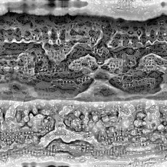 or his Turing Flow series:

McCabe’s images are created using a more complex multi-scale model. Softology’s blog entry and W:Blut’s post dissect McCabe’s approach (there is even a reference implementation in Processing). Notice, that Nervous System sells some of McCabe’s works as jigsaw puzzles.
Reaction-Diffusion systems in WebGL
Felix Woitzel (@Flexi23) has created some beautiful WebGL-based reaction-diffusion demos, such as this Fluid simulation with Turing patterns:

He also has created several other RD based variants over at WebGL Playground.

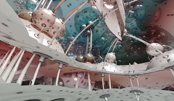
Fabricated 3D Objects
Jessica Rosenkrantz and Jesse Louis-Rosenberg at Nervous System create and sell objects designed and inspired by generative processes. Several of their objects, including these cups, plates, and lamps are based on reaction-diffusion systems, and can be bought from their webshop.

Be sure to read their blog entries about reaction-diffusion. And don’t forget to take a look at their Cell Cycle WebGL design app, while visiting.
Reaction-Diffusion Software
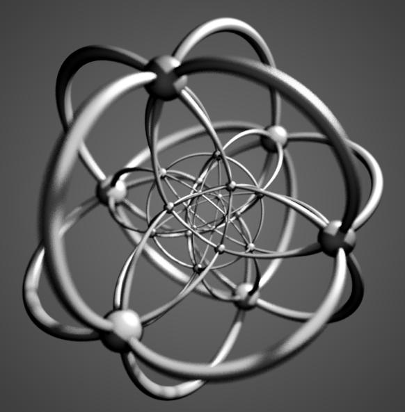
An easy way to explore reaction-diffusion systems with doing any coding is by using Ready, which uses OpenCL to explore RD systems. It has several interesting features, including the ability to run systems on 3D meshes and directly interact and ‘paint’ on the surfaces.

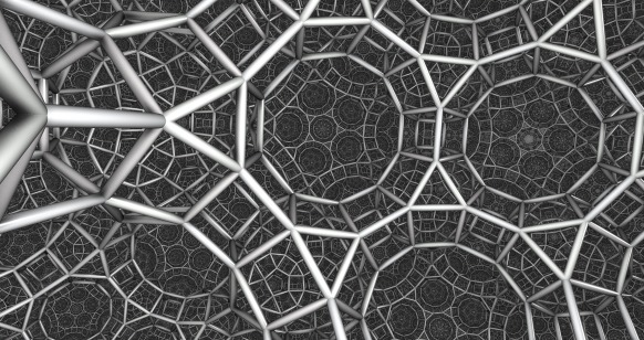
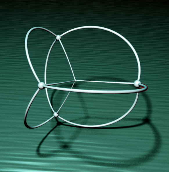
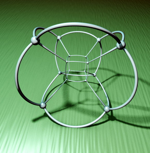
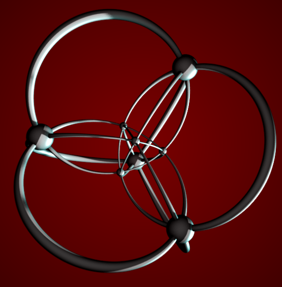
It also lets you run Game-of-Life on exotic geometries, such as a torus or even something as exotic as a Penrose tiling.