Yearly Archives: 2012

Fragmentarium 0.9.1 (“Chiaroscuro”) Released

I’ve released a new build of Fragmentarium, version 0.9.1 (“Chiaroscuro”).
It can be downloaded at Github (as of now only Windows builds are available).

The usual caveats apply: Fragmentarium is very much work in progress, and is best suited for people who like to experiment with code.

Dual buffers

The main new feature is support for dual buffers and dual shaders. The front buffer is swapped after each frame to the backbuffer, which can be accessed as: ‘uniform sampler2D backbuffer;’.

Buffers can be created as either 8-bit or 16-bit integer, or 32-bit float. The new buffers makes it possible to create accumulated ray tracing, high quality AA for 2D systems, and many types of feedback systems. The easiest way to start exploring these features is by looking at the new tutorials (see below).


Minor improvements:

  • Changed UI a bit to make it easier to change from automatic to continuous rendering.
  • Added context menu option to insert preset based on current settings.
  • The syntax for using ‘2D.frag’ is simpler now. Just implement: “vec3 color(vec2 c);”
  • Bugfix: Fixed error in 2D.frag, where changing aspect ratio would mess up viewport translation.
  • Bugfix: Fixed some errors in the included fragments: Noise, Tetrahedron, and several of Knighty’s examples were missing a ‘providesInit’.
  • Bugfix: Fixed specular bug in standard-raytracer.
  • Bugfix: Copying from web was sometimes weird (should now strip rich text).
  • Bugfix: Autosave files now creates a directory with output files (necessary since the #BufferShader directive broke the old ‘include all in one file’ system).


New fragments:

  • Added a new ‘tutorial’ category, with examples of many features in Fragmentarium.
  • Soft-Raytracer.frag – An example progressive (accumulated) ray-tracer. DOF using finite aperture, HDR and tonemapping, soft shadows, and multiple ray ambient occlusion, and sub-pixel jittered high-quality anti-alias. All very experimental.
  • Progressive2D.frag, Progressive2DJulia.frag – Can be used for high-quality (progressive) anti-alias of 2D systems. Uniform disk sampling, Gaussian and Box filtering, “gamma correct” averaging of samples.
  • A Quilez inspired ‘Domain Distortion’ example.
  • A dual-buffered Game of Life example.
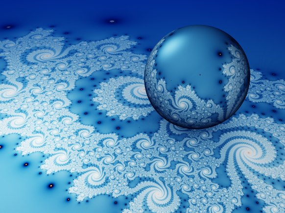
  • Mandelbrot Averaged Stripe Coloring example.
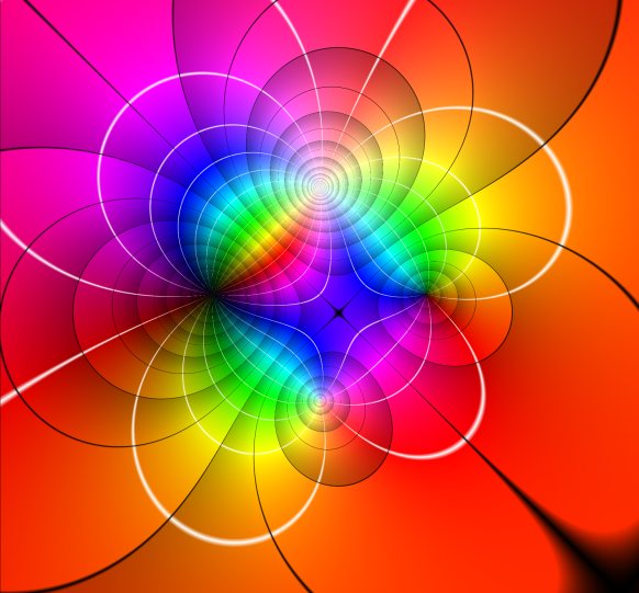
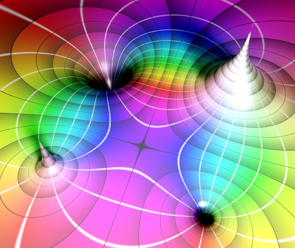
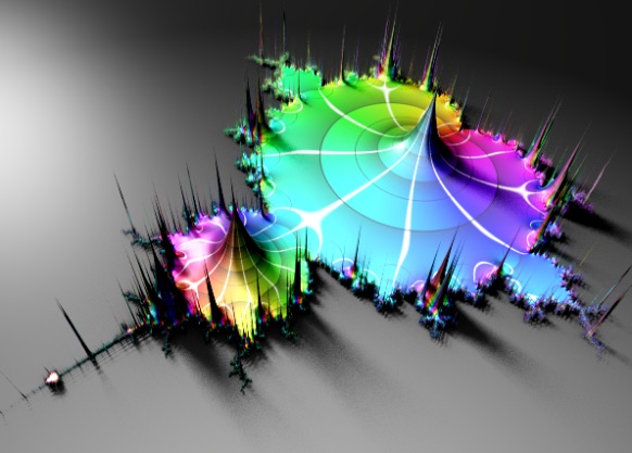
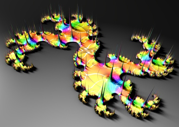
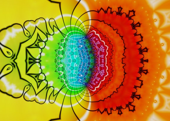
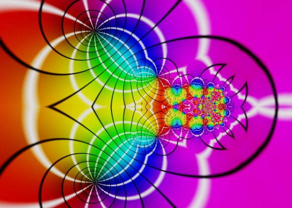
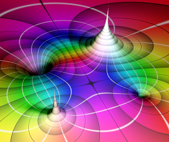
  • Lifted Domain Coloring example (in 2D/3D), see here.
  • New ‘Theory’ category with examples of the dual number and automatic differentiation method.
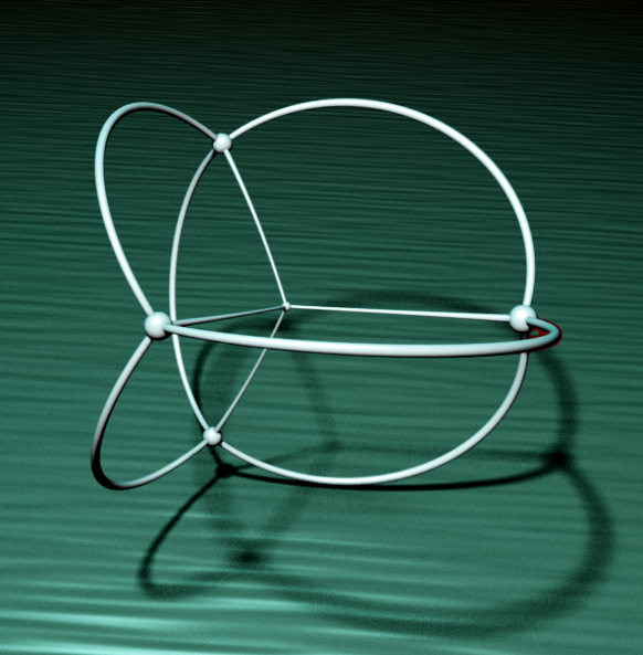
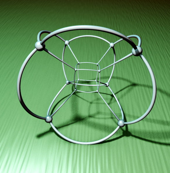
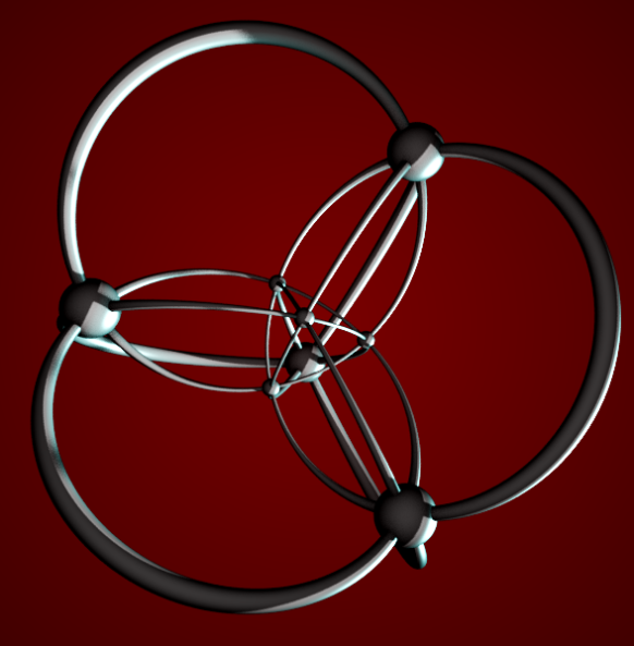
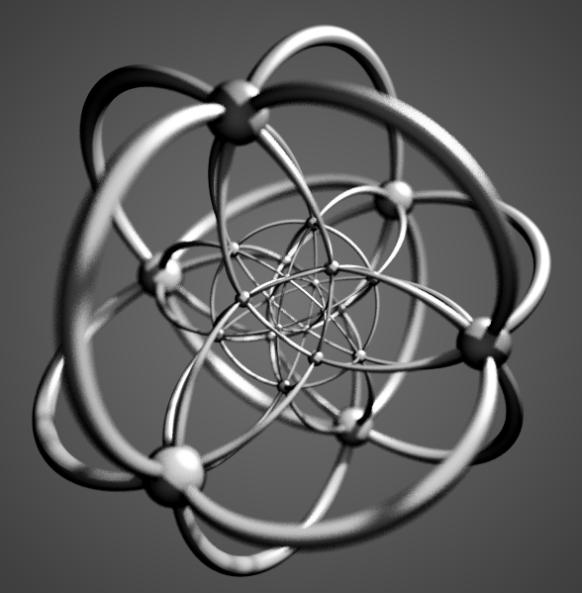
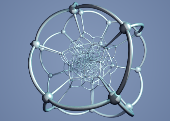
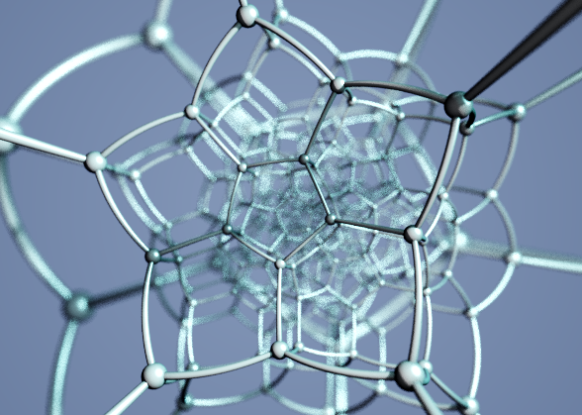
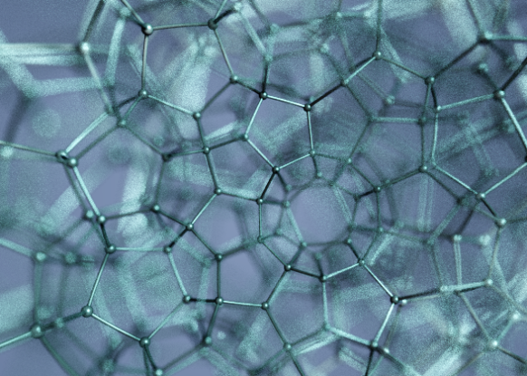
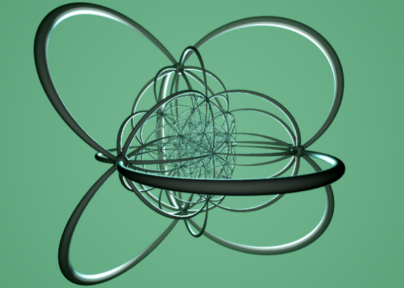
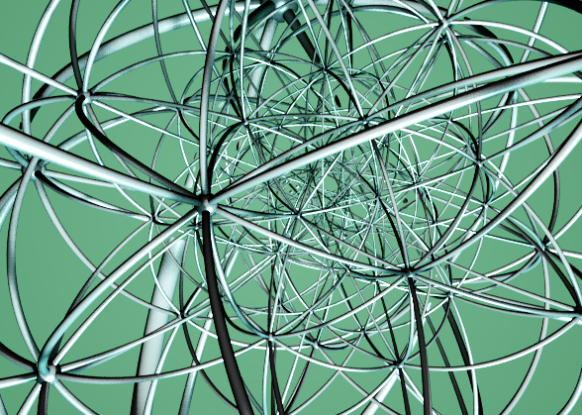
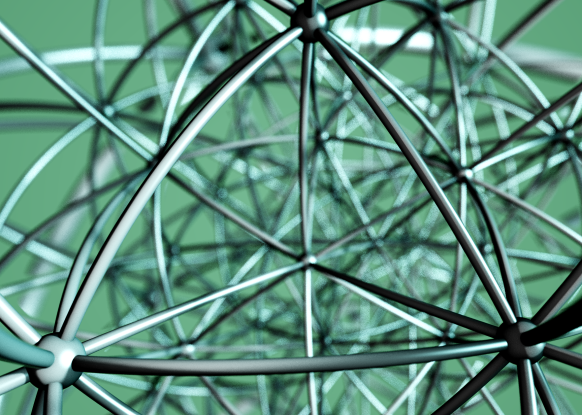
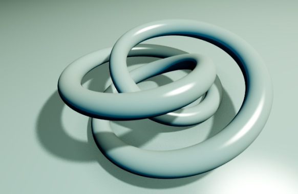
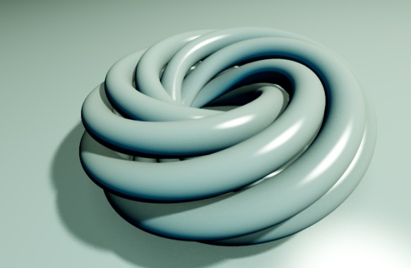
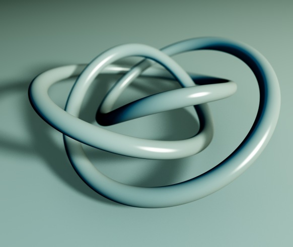
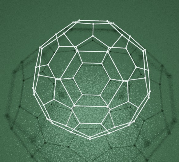
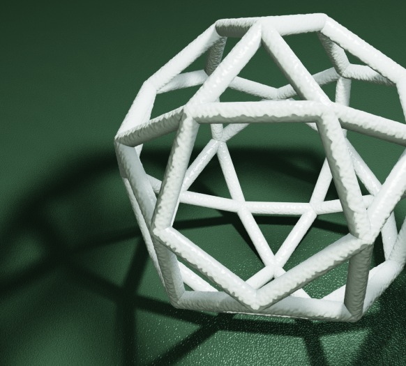
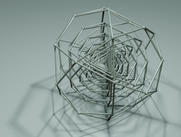
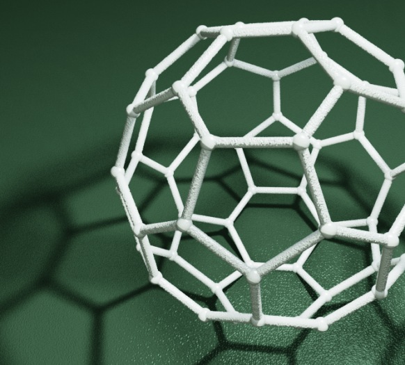
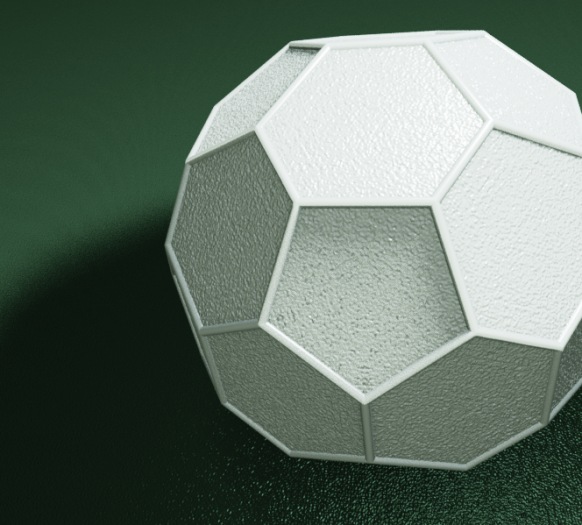
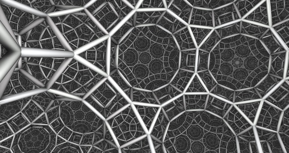
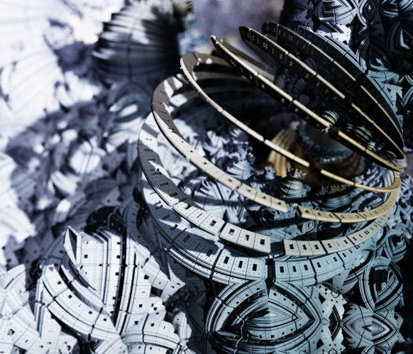
  • Some great new scripts from Knighty, for polyhedrons, knots, polychora, and hyperbolic tesselations. See here and here.

ATI users

Some fragments fail on ATI cards. This seems to be due to faulty GLSL driver optimizations. A workaround is to lock the ‘iterations’ variable (click the padlock next to it). Adding a bailout check inside the main DE loop (e.g. ‘if (length(z)>1000.0) break;’) also seems to do the job. I don’t own an ATI card, so I cannot debug this without people helping.

Mac users

Some Mac users has reported problems with the last version of Fragmentarium. Again, I don’t own a Mac, so I cannot solve these issues without help.

Finally, please read the FAQ, before asking questions.

For more examples of images generated with the new version, take a look at the Flickr Fragmentarium stream.

Spherical Worlds

Recently I saw a description of spherical fractals in a blog post by Samuel Monnier.

These Julia-sets are constructed like ordinary Mandelbrots and Julias: first the argument is squared, but instead of adding a constant afterwards, a Möbius transformation is applied:

\(z = \frac{a z^2 + b}{c z^2 + d}\)

For the right choices of (complex) constants, plane-filling patterns appear.

There is an intimate connection between Möbius transformations and spherical geometry: if the plane is stereographically projected onto a sphere, a Möbius transformations corresponds to rotating and moving the sphere, and then project stereographically back to the plane (this is nicely visualized in this video).


This connection can be visualized graphically: if the plane-filling patterns are stereographically projected onto a sphere, they fit naturally on it. There are no discontinuities or voids, and no singularities near the poles.


Here I’ve used Fragmentarium to create some images of these plane-filling patterns, together with their stereographical projection onto a sphere. It was done by distance estimated ray marching, but in this case we could have used ordinary ray tracing, and calculated the exact intersections.


The Fragmentarium script can be found here.

Lifted Domain Coloring

This year, one of the pictures at the International Science & Engineering Visualization Challenge, caught my interest.

Poelke and Polthier’s Lifted Domain Coloring is a coloring scheme for visualizing properties of complex functions: it maps numbers in the complex plane stereographically to the Riemann sphere, and assigns a hue based on the inclination angle (though I’m not sure that much is gained by the stereographic projection, since the polar representation of the complex numbers seems to provide all the needed information). Saturation and Brightness are controlled by the modulus of the number: when the modulus goes towards infinity, the color turns white, and for numbers close to zero, the color turns black. The exact radial mapping used by the authors is not specified in the paper, but I think my implementation is quite close:

The visualization scheme makes it possible to visually identify different properties, such as zeroes and poles in complex functions.

One of the ways, I think such a visualization may be improved is by using a heightmap:

Here I’ve raised the poles and lowered the zeroes: first, I made the poles and zeroes appear symmetric, by transforming the modulus: r = abs(r + 1/r). Then I applied a sigmoid function to tame the infinities, and finally another sigmoid transformation was applied to change the sign of the zeroes. This technique will only work for somewhat well-behaved functions (meromorph functions – functions with a countable number of zeroes and poles).

Of course, I’ve also tested the Lifted Domain Coloring scheme on fractals.

Here is a Mandelbrot and Julia plot:

Usually Mandelbrot visualizations focus on coloring the outside of the set, but since the exterior of the Mandelbrot set has infinite modulus, only the interior (with its zeroes) are visualized here. The zeroes are visualized as peaks for better graphical clarity.

I also tested the coloring scheme on Samuel Monnier’s Ducks fractal:


Here, the coloring scheme does a decent job for low iteration counts, but for higher iterations the images become messy, so for pure aestethic purposes there are probably better coloring schemes around.

Distance Estimated Polychora

My last post mentioned some scripts that Knighty (a Fractal Forums member) made for distance estimated rendering of many types of polyhedra, including the Platonic solids. Shortly after, Knighty really raised the bar by finding a distance estimator for four dimensional polytopes. In this post, I’ll show some images of a subset of these, the convex regular polychora.

There are several ways to depict four dimensional structures. The 4D Quaternion Julia, one of the first distance estimated fractals, simply showed 3D slices of 4D space. Another way would be to project the shadow of a 4D object onto a 3D space. Ideally, a proper perspective projective would be preferable, but this seems to be complicatated with distance estimation techniques.

The technique Knighty used to create a 3D projection, was to place the polychoron boundary on a 3-sphere, and then stereographically project the 3-sphere surface onto a 3-dimensional space. For a very thorough and graphical introduction to stereographic projection of higher-dimensional polytopes, see this great movie: Dimensions. It should be noted that the Jenn3D program also uses this projection to depict a variety of polytopes (using polygonal rendering, not distance estimated ray marching).

Back to the structures:

The convex regular 4-polytopes are the four-dimensional analogs of the Platonic solids. They are bounded by three-dimensional cells, which are all Platonic solids of the same kind (similar to the way the Platonic solids are bounded by identical regular 2D polygons). The convex regular polytopes are consistently named by the number of identical cells (Platonic solids) that bounds them. In four dimensions, there are six of these, one more than the number of Platonic solids.

5-cell

The 5-cell (or 4-simplex, or hypertetrahedron) is the simplest of the convex regular polytopes. It is composed of 5 three-dimensional tetrahedrons, resulting in a total of 5 vertices and 10 edges. It is the 4D generalisation of a tetrahedron.

The curved lines are a consequence of the stereographic projection. In 4D the lines would be straight.

8-cell

The 8-cell (or hypercube, or Tesseract) is also simple. Composed of 8 3D-cubes, it has 16 vertices, and 32 edges. It is the 4D generalisation of a cube.

16-cell

Things start to get more complicated with the 16-cell (or hyperoctahedron). It is composed of 16 tetrahedrons, and has 8 vertices and 24 edges. It is the 4D generalisation of an octahedron.

Notice, that if we rotate the 3-sphere, we can get interesting depictions, with edges getting infinitely long in 3-space:

24-cell

The 24-cell is exceptional, since it has no 3D analogue. It is built from 24 octahedrons, has 24 vertices and 96 edges.

120-cell

The 120-cell is a beast, built from 120 three-dimensional dodecahedra. With 600 vertices and 1200 edges, it is the most complex of the convex, regular polychora. It is the 4D generalisation of a dodecahedron.

Zooming in, it is easier to see the pentagons making up the dodecahedra.

600-cell

Finaly, the 600-cell is built from an even larger number of polyhedra: 600 three-dimensional tetrahedrons. However, the simpler polyhedra means there is only a total of 120 vertices and 720 edges. It is the 4D generalisation of an icosahedron.

Knighty’s great Fragmentarium scripts can be found in this thread at Fractal Forums.

Knighty’s script is not limited to regular convex polychora. Many types of polytopes can be made. Here are the parameters used for the images in this post:

polychora06.frag parameters:

Type,U,V,W,T
3,0,1,0,0 - 5-cell
4,0,1,0,0 - 8-cell
4,0,0,1,0 - 24-cell
4,0,0,0,1 - 16-cell
5,0,1,0,0 - 120-cell
5,0,0,0,1 - 600-cell

And for completeness, here are the parameters for the 3D polyhedron script:

Type,U,V,W
3,0,1,0 Tetrahedron
4,0,0,1 Cube
3,1,0,0 Octahedron
5,0,0,1 Dodecahedron
5,0,1,0 Icosahedron

Knots and Polyhedra

Over at Fractal Forums, DarkBeam came up with a Distance Estimator for a trefoil knot in this thread. Here are a few samples, created using the new ‘soft’ raytracer, I’m working on in Fragmentarium:

These kinds of knots are easy to describe by a parametrized curve, but making a distance estimator for them is impressive – I wouldn’t have guessed it was possible at all.

It is also possible to create several variations:

In the same thread, Knighty came up with an impressive figure-8 knot distance estimator:

In another thread at Fractal Forums, Knighty also published an interesting technique (“Fold and Cuts”) for creating a large variety of distance estimated polyhedra:

(If you wonder about the materials, I’ve added some 3D Perlin noise to the distance estimate – this is simple way to creature a structural texture, and it creates true displacements, not just surface normal perturbations).

The threads linked to above contains Fragmentarium scripts with the relevant distance estimators.