During the last two years, the 3D fractal field has undergone a small revolution: the Mandelbulb (2009), the Mandelbox (2010), The Kaleidoscopic IFS’s (2010), and a myriad of equally or even more interesting hybrid systems, such as Spudsville (2010) or the Kleinian systems (2011).

All of these systems were made possible using a technique known as Distance Estimation and they all originate from the Fractal Forums community.

Overview of the posts

Part I briefly introduces the history of distance estimated fractals, and discuss how a distance estimator can be used for ray marching.

Part II discuss how to find surface normals, and how to light and color fractals.

Part III discuss how to actually create a distance estimator, starting with distance fields for simple geometric objects, and talking about instancing, combining fields (union, intersections, and differences), and finally talks about folding and conformal transformation, ending up with a simple fractal distance estimator.

Part IV discuss the holy grail: the search for generalization of the 2D (complex) Mandelbrot set, including Quaternions and other hypercomplex numbers. A running derivative for quadratic systems is introduced.

Part V continues the discussion about the Mandelbulb. Different approaches for constructing a running derivative is discussed: scalar derivatives, Jacobian derivatives, analytical solutions, and the use of different potentials to estimate the distance.

Part VI is about the Mandelbox fractal. A more detailed discussion about conformal transformations, and how a scalar running derivative is sufficient, when working with these kind of systems.

Part VII discuss how dual numbers and automatic differentation may used to construct a distance estimator.

Part VIII is about hybrid fractals, geometric orbit traps, various other systems, and links to relevant software and resources.

The background

The first paper to introduce Distance Estimated 3D fractals was written by Hart and others in 1989:
Ray tracing deterministic 3-D fractals

In this paper Hart describe how Distance Estimation may be used to render a Quaternion Julia 3D fractal. The paper is very well written and definitely worth spending some hours on (be sure to take a look at John Hart’s other papers as well). Given the age of Hart’s paper, it is striking that is not until the last couple of years that the field of distance estimated 3D fractals has exploded. There has been some important milestones, such as Keenan Crane’s GPU implementation (2004), and Iñigo Quilez 4K demoscene implementation (2007), but I’m not aware of other fractal systems being explored using Distance Estimation, before the advent of the Mandelbulb.

Raymarching

Classic raytracing shoots one (or more) rays per pixel and calculate where the rays intersect the geometry in the scene. Normally the geometry is described by a set of primitives, like triangles or spheres, and some kind of spatial acceleration structure is used to quickly identify which primitives intersect the rays.

Distance Estimation, on the other hand, is a ray marching technique.

Instead of calculating the exact intersection between the camera ray and the geometry, you proceed in small steps along the ray and check how close you are to the object you are rendering. When you are closer than a certain threshold, you stop. In order to do this, you must have a function that tells you how close you are to the object: a Distance Estimator. The value of the distance estimator tells you how large a step you are allowed to march along the ray, since you are guaranteed not to hit anything within this radius.

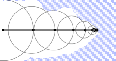
Schematics of ray marching using a distance estimator.

The code below shows how to raymarch a system with a distance estimator:

float trace(vec3 from, vec3 direction) {
	float totalDistance = 0.0;
	int steps;
	for (steps=0; steps < MaximumRaySteps; steps++) {
		vec3 p = from + totalDistance * direction;
		float distance = DistanceEstimator(p);
		totalDistance += distance;
		if (distance < MinimumDistance) break;
	}
	return 1.0-float(steps)/float(MaxRaySteps);
}

Here we simply march the ray according to the distance estimator and return a greyscale value based on the number of steps before hitting something. This will produce images like this one (where I used a distance estimator for a Mandelbulb):

It is interesting that even though we have not specified any coloring or lighting models, coloring by the number of steps emphasizes the detail of the 3D structure - in fact, this is an simple and very cheap form of the Ambient Occlusion soft lighting often used in 3D renders.

Parallelization

Another interesting observation is that these raymarchers are trivial to parallelise, since each pixel can be calculated independently and there is no need to access complex shared memory structures like the acceleration structure used in classic raytracing. This means that these kinds of systems are ideal candidates for implementing on a GPU. In fact the only issue is that most GPU's still only supports single precision floating points numbers, which leads to numerical inaccuracies faster than for the CPU implementations. However, the newest generation of GPU's support double precision, and some API's (such as OpenCL and Pixel Bender) are heterogeneous, meaning the same code can be executed on both CPU and GPU - making it possible to create interactive previews on the GPU and render final images in double precision on the CPU.

Estimating the distance

Now, I still haven't talked about how we obtain these Distance Estimators, and it is by no means obvious that such functions should exist at all. But it is possible to intuitively understand them, by noting that systems such as the Mandelbulb and Mandelbox are escape-time fractals: we iterate a function for each point in space, and follow the orbit to see whether the sequence of points diverge for a maximum number of iterations, or whether the sequence stays inside a fixed escape radius. Now, by comparing the escape-time length (r), to its spatial derivative (dr), we might get an estimate of how far we can move along the ray before the escape-time length is below the escape radius, that is:

\(DE = \frac{r-EscapeRadius }{dr}\)
 
This is a hand-waving estimate - the derivative might fluctuate wildly and get larger than our initial value, so a more rigid approach is needed to find a proper distance estimator. I'll a lot more to say about distance estimators inthe later posts, so for now we will just accept that these function exists and can be obtained for quite a diverse class of systems, and that they are often constructed by comparing the escape-time length with some approximation of its derivative.

It should also be noticed that this ray marching approach can be used for any kinds of systems, where you can find a lower bound for the closest geometry for all points in space. Iñigo Quilez has used this in his impressive procedural SliseSix demo, and has written an excellent introduction, which covers many topics also relevant for Distance Estimation of 3D fractals.

This concludes the first part of this series of blog entries. Part II discusses lighting and coloring of fractals.