Previous parts: part I, part II, part III, part IV and part V.
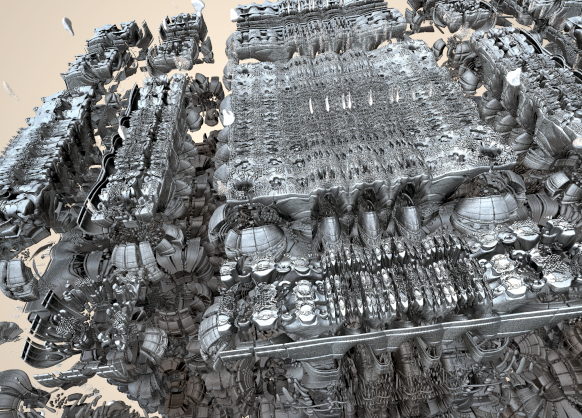
After the Mandelbulb, several new types of 3D fractals appeared at Fractal Forums. Perhaps one of the most impressive and unique is the Mandelbox. It was first described in this thread, where it was introduced by Tom Lowe (Tglad). Similar to the original Mandelbrot set, an iterative function is applied to points in 3D space, and points which do not diverge are considered part of the set.
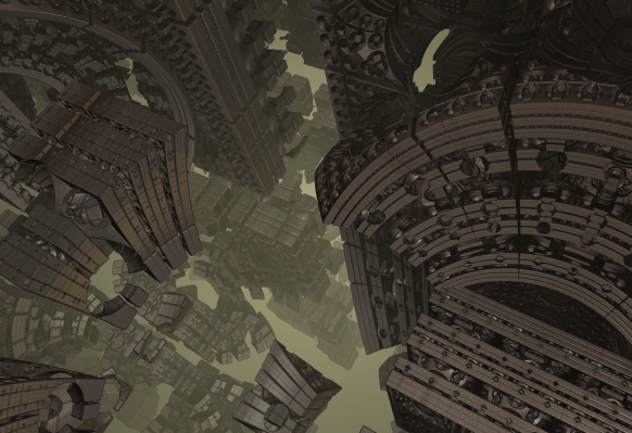
Tom Lowe has a great site, where he discusses the history of the Mandelbox, and highlights several of its properties, so in this post I’ll focus on the distance estimator, and try to make some more or less convincing arguments about why a scalar derivative works in this case.
The Mandelbulb and Mandelbrot systems use a simple polynomial formula to generate the escape-time sequence:
\(z_{n+1} = z_n^\alpha + c\)The Mandelbox uses a slightly more complex transformation:
\(z_{n+1} = scale*spherefold(boxfold(z_n)) + c\)I have mentioned folds before. These are simply conditional reflections.
A box fold is a similar construction: if the point, p, is outside a box with a given side length, reflect the point in the box side. Or as code:
if (p.x>L) { p.x = 2.0*L-p.x; } else if (p.x<-L) { p.x = -2.0*L-p.x; }
(this must be done for each dimension. Notice, that in GLSL this can be expressed elegantly in one single operation for all dimensions: p = clamp(p,-L,L)*2.0-p)
The sphere fold is a conditional sphere inversion. If a point, p, is inside a sphere with a fixed radius, R, we will reflect the point in the sphere, e.g:
float r = length(p);
if (r<R) p=p*R*R/(r*r);
(Actually, the sphere fold used in most Mandelbox implementations is slightly more complex and adds an inner radius, where the length of the point is scaled linearly).
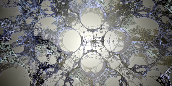
Now, how can we create a DE for the Mandelbox?
Again, it turns out that it is possible to create a scalar running derivative based distance estimator. I think the first scalar formula was suggested by Buddhi in this thread at fractal forums. Here is the code:
float DE(vec3 z)
{
	vec3 offset = z;
	float dr = 1.0;
	for (int n = 0; n < Iterations; n++) {
		boxFold(z,dr);       // Reflect
		sphereFold(z,dr);    // Sphere Inversion

                z=Scale*z + offset;  // Scale & Translate
                dr = dr*abs(Scale)+1.0;
	}
	float r = length(z);
	return r/abs(dr);
}
where the sphereFold and boxFold may be defined as:
void sphereFold(inout vec3 z, inout float dz) {
	float r2 = dot(z,z);
	if (r<minRadius2) {
		// linear inner scaling
		float temp = (fixedRadius2/minRadius2);
		z *= temp;
		dz*= temp;
	} else if (r2<fixedRadius2) {
		// this is the actual sphere inversion
		float temp =(fixedRadius2/r2);
		z *= temp;
		dz*= temp;
	}
}

void boxFold(inout vec3 z, inout float dz) {
	z = clamp(z, -foldingLimit, foldingLimit) * 2.0 - z;
}
It is possible to simplify this even further by storing the scalar derivative as the fourth component of a 4-vector. See Rrrola’s post for an example.
However, one thing that is missing, is an explanation of why this distance estimator works. And even though I do not completely understand the mechanism, I’ll try to justify this formula. It is not a strict derivation, but I think it offers some understanding of why the scalar distance estimator works.
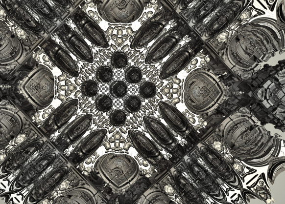
A Running Scalar Derivative
Let us say, that for a given starting point, p, we obtain an length, R, after having applied a fixed number of iterations. If the length is less then \(R_{min}\), we consider the orbit to be bounded and is thus part of the fractal, otherwise it is outside the fractal set. We want to obtain a distance estimate for this point p. Now, the distance estimate must tell us how far we can go in any direction, before the final radius falls below the minimum radius, \(R_{min}\), and we hit the fractal surface. One distance estimate approximation would be to find the direction, where R decreases fastest, and do a linear extrapolation to estimate when R becomes less than \(R_{min}\):
\(DE=(R-R_{min})/DR\)where DR is the magnitude of the derivative along this steepest descent (this is essentially Newton root finding).
In the previous post, we argued that the linear approximation to a vector-function is best described using the Jacobian matrix:
\(F(p+dp) \approx F(p) + J(p)dp
\)
The fastest decrease is thus given by the induced matrix norm of J, since the matrix norm is the maximum of \(|J v|\) for all unit vectors v.
So, if we could calculate the (induced) matrix norm of the Jacobian, we would arrive at a linear distance estimate:
\(DE=(R-R_{min})/\|J\|
\)
Calculating the Jacobian matrix norm sounds tricky, but let us take a look at the different transformations involved in the iteration loop: Reflections (R), Sphere Inversions (SI), Scalings (S), and Translations (T). It is also common to add a rotation (ROT) inside the iteration loop.
Now, for a given point, we will end applying an iterated sequence of operations to see if the point escapes:
\(Mandelbox(p) = (T\circ S\circ SI\circ R\circ \ldots\circ T\circ S\circ SI\circ R)(p)
\)
In the previous part, we argued that the most obvious derivative for a R^3 to R^3 function is a Jacobian. According to the chain rule for Jacobians, the Jacobian for a function such as this Mandelbox(z) will be of the form:
\(J_{Mandelbox} = J_T * J_S * J_{SI} * J_R …. J_T * J_S * J_{SI} * J_R
\)
In general, all of these matrices will be functions of R^3, which should be evaluated at different positions. Now, let us take a look of the individual Jacobian matrices for the Mandelbox transformations.
Translations
A translation by a constant will simply have an identity matrix as Jacobian matrix, as can be seen from the definitions.
Reflections
Consider a simple reflection in one of the coordinate system planes. The transformation matrix for this is:
\(T_{R} = \begin{bmatrix}
1 & & \\
& 1 & \\
& & -1
\end{bmatrix}
\)
Now, the Jacobian of a transformation defined by multiplying with a constant matrix is simply the constant matrix itself. So the Jacobian is also simply a reflection matrix.
Rotations
A rotation (for a fixed angle and rotation vector) is also constant matrix, so the Jacobian is also simply a rotation matrix.
Scalings
The Jacobian for a uniform scaling operation is:
\(J_S = scale*\begin{bmatrix}
1 & & \\
& 1 & \\
& & 1
\end{bmatrix}
\)
Sphere Inversions
Below can be seen how the sphere fold (the conditional sphere inversion) transforms a uniform 2D grid. As can be seen, the sphere inversion is an anti-conformal transformation – the angles are still 90 degrees at the intersections, except for the boundary where the sphere inversion stops.
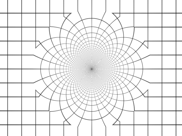
The Jacobian for sphere inversions is the most tricky. But a derivation leads to:
\(J_{R} = (r^2/R^2) \begin{bmatrix}
1-2x^2/R^2 & -2xy/R^2 & -2xz/R^2 \\
-2yx/R^2 & 1-2y^2/R^2 & -2yz/R^2 \\
-2zx/R^2 & -zy/R^2 & 1-2z^2/R^2
\end{bmatrix}
\)
Here R is the length of p, and r is radius of the inversion sphere. I have extracted the scalar front factor, so that the remaining part is an orthogonal matrix (as is also demonstrated in the derivation link).
Notice that all reflection, translation, and rotation Jacobian-matrices will not change the length of a vector when multiplied with it. The Jacobian for the Scaling matrix, will multiply the length with the scale factor, and the Jacobian for the Sphere Inversion will multiply the length by a factor of (r^2/R^2) (notice that the length of the point must evaluated at the correct point in the sequence).
Now, if we calculated the matrix norm of the Jacobian:
\(|| J_{Mandelbox} || = || J_T * J_S * J_{SI} * J_R …. J_T * J_S * J_{SI} * J_R ||
\)
we can easily do it, since we do only need to keep track of the scalar factor, whenever we encounter a Scaling Jacobian or a Sphere Inversion Jacobian. All the other matrix stuff will simply not change the length of a given vector and may be ignored. Also notice, that only the sphere inversion depends on the point where the Jacobian is evaluated – if this operation was not present, we could simply count the number of scalings performed and multiply the escape length with \(2^{-scale}\).
This means that the matrix norm of the Jacobian can be calculated using only a simply scalar variable, which is scaled, whenever we apply the scaling or sphere inversion operation.
This seems to hold for all conformal transformations (strictly speaking sphere inversions and reflections are not conformal, but anti-conformal, since orientations are reversed). Wikipedia also mentions, that any function, with a Jacobian equal to a scalar times a rotational matrix, must be conformal, and it seems the converse is also true: any conformal or anti-conformal transformation in 3D has a Jacobian equal to a scalar times a orthogonal matrix.
Final Remarks
There are some reasons, why I’m not completely satisfied why the above derivation: first, the translational part of the Mandelbox transformation is not really a constant. It would be, if we were considering a Julia-type Mandelbox, where you add a fixed vector at each iteration, but here we add the starting point, and I’m not sure how to express the Jacobian of this transformation. Still, it is possible to do Julia-type Mandelbox fractals (they are quite similar), and here the derivation should be more sound. The transformations used in the Mandelbox are also conditional, and not simple reflection and sphere inversions, but I don’t think that matters with regard to the Jacobian, as long as the same conditions are used when calculating it.
Update: As Knighty pointed out in the comments below, it is possible to see why the scalar approximation works in the Mandelbrot case too:
Let us go back to the original formula:
\(f(z) = scale*spherefold(boxfold(z)) + c\)
and take a look at its Jacobian:
\(J_f = J_{scale}*J_{spherefold}*J_{boxfold} + I\)
Now by using the triangle inequality for matrix norms, we get:
\(||J_f|| = ||J_{scale}*J_{spherefold}*J_{boxfold} + I|| \)
\(\leq ||J_{scale}*J_{spherefold}*J_{boxfold}|| + ||I|| \)
\(= S_{scale}*S_{spherefold}*S_{boxfold} + 1 \)
where the S’s are the scalars for the given transformation. This argument can also be applied to repeated applications of the Mandelbox transformation. This means, that if we add one to the running derivative at each iteration (like in the Mandelbulb case), we get an upper bound of the true derivative. And since our distance estimate is calculated by dividing with the running derivate, this approximation yields a smaller distance estimate than the true one (which is good).
Another point is, that it is striking that we end up with the same scalar estimator as for the tetrahedron in part 3 (except that is has no sphere inversion). But for the tetrahedron, the scalar estimator was based on straight-forward arguments, so perhaps it is possible to come up with a much simpler argument for the running scalar derivative for the Mandelbox as well.
There must also be some kind of link between the gradient and the Jacobian norm. It seems, that the norm of the Jacobian should be equal to the absolute value of the length of the Mandelbox(p) function: ||J|| = |grad|MB(p)||, since they both describe how fast the length varies along the steepest descent path. This would also make the link to the gradient based numerical methods (discussed in part 5) more clear.
And finally, if we reused our argumentation for using a linear zero-point approximation of the escape length to the Mandelbulb, it just doesn’t work. Here it is necessary to introduce a log-term (\(DE= 0.5*r*log(r)/dr\)). Of course, the Mandelbulb is not composed of conformal transformations, so the “Jacobian to Scalar running derivative” argument is not valid anymore, but we already have an expression for the scalar running derivative for the Mandelbulb, and this expression does not seem to work well with the \(DE=(r-r_{min})/dr\) approximation. So it is not clear under what conditions this approximation is valid. Update: Again, Knighty makes some good arguments below in the comments for why the linear approximations holds here.
The next part is about dual numbers and distance estimation.